Copyright © 1995-2001 MZA Associates Corporation

Anchoring WaveTrain to ACS using a DPE Test Case

WaveTrain is a highly reconfigurable wave optics modeling tool designed to serve the modeling needs of the ABL program, providing accurate performance prediction for a wide variety of HEL weapons systems and related experiments. To fill this role it is crucial to establish a high level of confidence in its correctness. Fortunately, there are a number of wave optics codes available which have already been anchored to experiment, so we need only anchor WaveTrain to one or more of these. We have recently completed our first anchoring exercise, in which we used WaveTrain to reproduce the results of ACS, written by Don Link of SAIC, in modeling the Differential Phase Experiment (DPE). This is a sensitive test of most of the basic wave optics modeling mechanisms, including point source modeling, Fourier propagation, spatial and frequency domain filtering, phase screen generation, interpolation, and post-processing algorithms. We used independently generated random phase screens, so we compared the results on a statistical basis. Specifically, we computed the irradiance variance at the receiver aperture for each source and the differential phase variance, using two different beacon separations and three different turbulence strengths, computing 40 Monte Carlo realizations for each case. We also tried two different interpolation methods, bilinear and cubic; for cubic interpolation in WaveTrain we reproduced the precise algorithm used in ACS. Our results were excellent: For each case, all quantities we compared matched to within the intrinsic estimate error due to finite sample size.

The simulation parameters are described in Table 1.

For each beacon, the complex field was initialized with a single nonzero mesh point, at the (n/2+1, n/2+1) point. The vertical beacon was located at (0.0, 0.0) in x and y, while the horizontal beacon was located at (0.08, 0.0) or (0.31,0.0). For the horizontal beacon, a tilt was applied to the reference wave, so that it arrived at the aperture centered at (0.0, 0.0).

In the initial propagation, from the beacon to the first phase screen, a frequency domain filter was applied to limit the angular spread of the field. The exact form of the filter was a "raised cosine", unity in the center, zero at the edges, with a half cosine wave as transition. The full width of the nonzero region, expressed as an angle, was 1.5*nx*dx / z, while the width of the cosine transition regions on either side were 0.05*nx*dq, where dq = l / (nx*dx). After completing the propagation, a spatial domain filter, also a raised cosine, was applied. In this case, the full width of the nonzero region was 0.9*nx*dx, while the transition regions were .05*nx*dx. On the second and subsequent propagations a different frequency domain filter was used, where the width of the transition regions was unchanged, while the width of the nonzero region was 0.95*nx*dq. The same spatial domain filter was used in each propagation.

After each propagation, a phase screen was applied to the field. For the vertical beam, the screen grid and the propagation grid were aligned. For the horizontal beam, the meshes were aligned in one dimension but not in the other, so it was necessary to interpolate the screen onto the propagation mesh. Two different interpolation algorithms were tried, bilinear and cubic. The specific cubic interpolation algorithm used was taken from ACS; the weight function is separable in x and y, and the weights, w_i, are given by the following:

w₀ = -(1/3)r + (1/2)r2 -(1/6)r3

w₁ = 1 -(1/2)r - r2 +(1/2)r3

w₂ = r + (1/2)r2 -(1/2)r3

w₃ = -(1/6)r +(1/6)r3

where x₁ <= x < x₂, y₁ <= y < y₂, and r = (x-x₁)/dx or (y-y₁)/dy.

For each turbulence strength and beacon separation we generated forty Monte Carlo realizations each with WaveTrain and ACS, and recorded the fields from each beacon for each iteration. To compare the statistics of the fields, for each iteration we computed the frame-normalized irradiance for each beacon, and the differential phase variance. We averaged the results over the forty realizations, then took the difference between corresponding WaveTrain and ACS results. Finally, we computed the expected estimate error due to finite sample size from the sample standard deviations, and divided the differences by that amount. Assuming the differences are entirely due to finite sampling, we would expect these ratios to be roughly unity; to be precise, the expected value of the squared magnitudes would be unity. Our results are consistent with this hypothesis. Furthermore, in the course of this exercise we learned that even very minor changes in the simulation parameters, e.g. a using a slightly different aperture function or filter, would be enough to destroy agreement at this level of detail. Because of this, and also because we painstakingly stepped through both simulations side-by-side, comparing results at each stage, we are convinced that WaveTrain is now well anchored to ACS with respect to all modeling components used in modeling DPE. There are additional components not used in DPE which remain to be anchored; we are preparing to do so.

The results of our comparisons are given in Tables 2 through 4. All the results shown were obtained using bilinear interpolation because we found that the choice of interpolation algorithm (bilinear or cubic) had very little effect, more than an order of magnitude (in variance) below the error due to finite sample size.

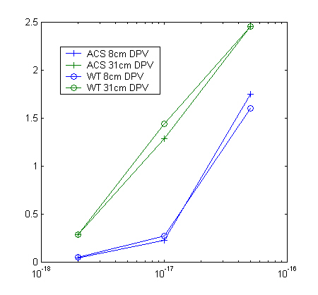
Figure 1: Differential phase variance vs. C_n²

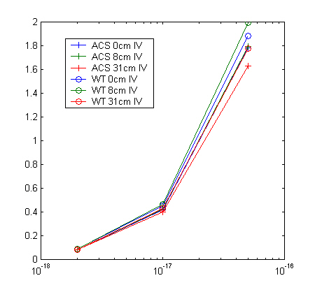
Figure 2: Normalized irradiance variance vs. C_n²

In the course of this exercise we learned a painful but useful lesson that will benefit us in future anchoring work. At the outset, we asked Don Link of SAIC to use ACS to construct a model of DPE and to prepare a detailed write-up to guide us in constructing a corresponding model in WaveTrain. We relied upon his write-up rather than the ACS source code and input files, and this proved to be a mistake, for two reasons: First, given that the modeling information already existed in a precise and unambiguous form, translating it into another form created an unnecessary opportunity for error, through typos and/or miscommunication. Second, we had no means to catch such errors at an early stage, and instead had to attempt diagnosis from the simulation results, where a simple error might have a non-obvious effect. Late in the exercise we switched tactics, invested the effort to understand ACS in more detail at the source code level, and started using side-by-side, step-by-step comparison. We were then able to finish the exercise in a relatively short time.