TurbTool is a Matlab GUI application that complements the WaveTrain wave-optics simulation code. TurbTool can also be used independently of WaveTrain. TurbTool serves essentially two purposes:

(1) TurbTool allows the user to specify a propagation geometry with turbulence strength and wind profiles, and then to very quickly compute analytic approximations to important integrated turbulence quantities. Examples of such quantities are scintillation irradiance variance, Fried's wave coherence length, isoplanatic angle, and the Greenwood and Tyler frequencies. This type of calculation is useful independent of or in concert with a WaveTrain wave-optics simulation. TurbTool also provides information regarding atmospheric scattering and absorption profiles along the propagation path.

(2) TurbTool can be used to generate a data file of phase-screen specifications that can serve as a complete set of arguments to WaveTrain's atmospheric specification modules. Such data may comprise turbulence screen locations, strengths and wind speeds, as well as absorption and scattering coefficients for companion thermal blooming screens. If so directed, TurbTool will save the required vectors to a *.mat file, which can later be read into a WaveTrain runset.

Function (1) of TurbTool allows the user to assess certain general behaviors to be expected from a given propagation geometry, and to quickly obtain parameters that may be used as checks on the detailed wave-optics simulation results. However, note that the integrated-turbulence formulas evaluated by TurbTool are either Rytov- or geometric-theory approximations. Therefore, one should expect agreement between simulation results and TurbTool predictions only within the domains of validity of the approximate formulas. The formulas used by TurbTool are specified later in this document.

Function (2) of TurbTool can be applied in several variations, as the user finds most helpful. As noted above, TurbTool can generate a data file containing the complete information required to specify atmospheric phase screens (turbulence and thermal blooming). This file can then be read in as a unit to the WaveTrain modules that require the information. However, users may prefer to use TurbTool to compute required data vectors (e.g., screen positions and C_n² values for AcsAtmSpec), and then to copy the data manually to various lines of a WaveTrain runset editor. While the latter procedure may involve a little more manual labor, some users may find that it provides a greater sense of user control and later readability of the runset. In any case, this is the most flexible way of using TurbTool-generated data as WaveTrain input.

In general, TurbTool can provide the user considerable help in generating WaveTrain atmospheric input data. TurbTool features include:

(1) Availability of numerous "standard" C_n² profiles (Clear-1, HV5/7, etc.) and wind profiles used by the community.

(2) Computation of effective, i.e. segment-average, C_n² values to be associated with discrete screens.

(3) Several standard options for generating path segmentation to define phase screen strengths, and to position the screens within the corresponding segments.

(4) Absorption and scattering data for thermal blooming screens, where this data is derived from the validated MODTRAN and FASCODE codes (developed at the Air Force Geophysics Laboratory).

(5) Continuous and discrete integration options for computing integrated turbulence quantities. These can be used to estimate the discretization effects of the split-step or lumped-parameter modeling of atmospheric propagation that is used in wave-optics simulation.

(6) Ability to define completely user-specified discrete profiles.

2 Starting TurbTool

(1) Open a Matlab session

(2) Make the current directory
C:\Program Files\mza\wavetrain\v2007a\mfiles\turb2007.tbx
Or, ensure that turb2007.tbx is the only turb*.tbx directory in the Matlab search path.
If you have a custom installation, adjust the above path to turb2007.tbx accordingly.

(3) At the Matlab prompt, type: >> turbtool
This will open the TurbTool main screen, whose appearance is shown in the following figure. (The numerical values shown here are the default startup values, except that Platform and Target Velocity have been altered from their default zeros).

(4) Depending on what other MZA software is present on your machine, you may receive (prior to the appearance of the Turbtool main screen) a dialog box asking whether the "pathtool" should attempt to find "ATMTools" and add that to your Matlab search path. If you do not have the ATMTools toolbox on your machine, then the absorption and scattering profiles will not be available in TurbTool. However, all the turbulence features of TurbTool will still be available.

Figure 1: Main screen of TurbTool GUI

3 Main screen inputs: General remarks

The main TurbTool screen contains the following principal elements:

(1) An input block where the optical propagation path geometry is specified. Above this block is a graphical representation of the propagation path.

(2) An input block where profile selections and parameters are specified.

(3) An input block where phase screen and miscellaneous parameters are specified. Above this block is a graphical representation of the discrete screen strengths and locations.

(4) An output table where computed values of integrated turbulence quantities are displayed.

(5) Status and informational blocks for display of certain messages.

(6) A set of pull-down menus to access further features.

Most input fields have Windows tool tips to quickly remind the user of key points: to see the tip, place the mouse pointer over the name of the input field.

3.1 Automatic recomputation

All output quantities on the main screen are immediately recomputed when any input specification is changed. After typing a revised number in an input field, the changes takes effect when the user (a) presses the <enter/return> key, or (b) places the cursor in another field.

3.2 Numerical notes and cautions

In certain circumstances, the order of computations combined with round-off produces a numerical singularity or a disallowed condition. An example is that the GUI sometimes reports that the minimum path altitude is below the earth's surface, even though it appears from the specified inputs that they are exactly equal. In such cases, the user is requested to slightly modify one of the inputs to avoid the singular condition. When such conditions occur, the problem should be obvious once the inputs are re-inspected.

4 Main screen inputs: Geometry

4.1 Color regions in the geometry plot

The figure panels (A) and (B) below show two examples of propagation path geometry. Note that four regions are color-coded in the companion plot. Dark blue represents the portion below mean sea level, light brown represents the portion between mean sea level and ground level, light blue represents the portion between ground level and the top of the turbulent atmosphere, and white represents the portion above the top of the turbulent atmosphere.

(A) (B)

Figure 2: Geometry input block: two path geometry examples

By default, the top of the turbulent atmosphere is defined as 50 km above mean sea level, but the user can change this by modifying a configuration file. Paths are allowed to have arbitrary portions above the turbulent atmosphere, but for computational purposes C_n² is set to zero there. (Note that even though C_n² is zero, these path portions still affect certain integrated turbulence quantities, because certain effects continue to evolve after a beam exits the turbulent region). Further details and the rationale for defining a top of the turbulent atmosphere are given in the sections that discuss turbulence profiles and integrated turbulence quantities.

In the propagation geometry plot, the lines that point from the P and T locations down through the mean sea level surface are always pointing to the center of the earth, as it would appear on the given plot scale. In other words, these lines are perpendicular to the sea-level surface in real space. However, if the plot scale is substantially different in the horizontal and vertical, the T line will appear to intersect the surface at an angle quite different from 90 degrees: this occurs because angles are not preserved in a mapping that has unequal horizontal and vertical scales.

4.2 Coordinate system

The optical propagation path is specified in terms of platform (P) and target (T) ends, where these terms have the same meaning as in WaveTrain. The significance of P(latform) and T(arget) within TurbTool and WaveTrain is:

(a) P(latform) is assigned the coordinate z = 0.

(b) T(arget) is assigned the coordinate z = L, where L the total propagation distance (slant range).

(c) In WaveTrain, outgoing waves define the +z direction, i.e., the P to T direction,
whereas incoming waves define the -z direction, i.e., the T to P direction. In TurbTool, "incoming" and "outgoing" tags are not used, except in reference to WaveTrain.

(d) Coordinate z is the slant-path linear coordinate between P (z = 0) and T (z = L). Matching the z orientations is significant when transferring data from TurbTool to WaveTrain run sets. Within TurbTool alone, there is no constraint on which path end is designated as having z = 0.

(e) P and T have no particular association with sources and sensors in TurbTool or WaveTrain (WaveTrain sources and sensors may be located at either or both P and T). Furthermore, TurbTool will automatically compute integrated turbulence quantities for both directions of propagation.

The two Cartesian axes transverse to z (the nominal propagation axis) are designated as the x and y axes. The role played by x and y in TurbTool is to provide references for specifying transverse velocities of platform, target and atmospheric wind. Other than forming an orthogonal triple, there is no constraint on how the user may orient the x and y directions. The orientation can be chosen to make the subsequent specification of x and y components of platform, target and atmospheric wind velocities as convenient as possible. The x,y orientation exists only in the user's head: the only specifications entered into TurbTool are the velocity components themselves. The velocity components affect some, but not all of the integrated turbulence quantities.

4.3 Path geometry inputs

TurbTool assumes a spherically-symmetric earth model. Input altitudes are specified along the local vertical, with respect to mean sea level (MSL). Path elevation angles at P or T are measured from the local horizontal (which is the line perpendicular to the local vertical). Allowed elevation angles are {-90 £ elev ang £ +90 deg}. The shorthand Platform(Target) Elev Angle that appears in the GUI means the elevation angle of the propagation path at the point P(T), with respect to the local horizontal at P(T), as illustrated in the figure below. In this example, the numerical value of P elev is positive, and the numerical value of T elev is negative.

Figure 3: Range and elevation angle definitions

A propagation path is defined by entering values for Ground Altitude, and then three of the six fields {Platform Altitude, Target Altitude, Platform Elevation Angle, Target Elevation Angle, Slant Range, Ground Range}. As soon as a complete set is specified, the program calculates the remaining dependent quantities. To specify a different set of input fields from the current selections, use the check boxes on the right side to first deselect current fields, and then to select the desired fields. Only the following input combinations are allowed:

	Allowed input combinations
1	P alt	slant R	T alt
2	P alt	ground R	T alt
3	P alt	P elev angle	slant R
4	P alt	P elev angle	ground R
5	T alt	T elev angle	slant R
6	T alt	T elev angle	ground R

Table 1: Allowed geometry input combinations

Physical units for all quantities are specified on the GUI screen.

4.4 Remarks on Ground Altitude

The first entry field in the GUI geometry block is Ground Altitude (with respect to mean sea level). The function of Ground Altitude in TurbTool is to cause certain adjustments in the standard turbulence strength vertical profiles. Details of this adjustment are described in the section on turbulence profiles. TurbTool assumes that the ground altitude under the propagation path is uniform.

4.5 Velocity inputs

Platform and target x and y velocities may be specified. The definition of the x and y axes is discussed in the section on coordinate systems. Platform and target velocities combine vectorially with the true wind profile to form a pseudo-wind profile that affects certain integrated turbulence results (the Greenwood and Tyler frequencies).

5 Main screen inputs: Profiles

The input block where profiles are specified is shown at right. Five types of profiles are currently supported: turbulence strength, wind speed, temperature, scattering coefficient, and absorption coefficient. Turbulence and wind specifications affect the integrated turbulence quantities reported in an output table. Scattering, absorption and temperature profiles do not affect the turbulence calculations in TurbTool. The scattering and absorption profiles only determine the optical transmissions reported in another output table. Additionally, the discrete values of scattering, absorption and temperature that are stored in a TurbTool output file (if such file is requested) may later be used by a WaveTrain run set to specify thermal blooming parameters.

The Scale input fields allows the user to apply an arbitrary multiplier factor to any selected profile. That is, the named profile values are multiplied by the same Scale factor at every point along the path. Wind is a vector, and therefore has two scale factors: this is discussed further in the section on wind profiles.

5.1 Turbulence profiles

TurbTool allows the user to: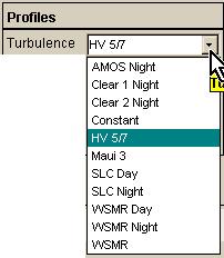
(a) select from a set of standard turbulence vertical profiles, or
(b) define a completely custom profile (discrete only).

As illustrated at right, by clicking the arrowhead at the right of the Turbulence list field, the user obtains a drop-down list of standard turbulence vertical profile names. Each of these profiles has achieved some recognition by researchers in the field of atmospheric propagation. Clicking on any profile name selects that profile. Notice that there is one profile named Constant , which implies C_n²= 1.0 m^-2/3 everywhere. This base value can then be scaled with the Scale factor entry.

A plot of the continuous turbulence profile may be inspected by using the menu option View - Turbulence profile (not View - Turbulence distribution ). For further background on some of the standard profiles, a good starting point is the article by Robert R. Beland, Propagation through Atmospheric Optical Turbulence, in Atmospheric Propagation of Radiation, The Infrared and Electro-Optical Systems Handbook, vol. 2, pp. 217-224, F.G. Smith, ed., ERIM and SPIE Press, 1993.

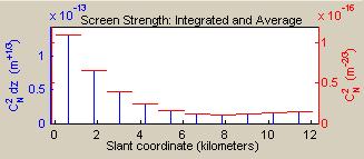A plot of the discrete turbulence distribution as represented by phase screens appears on the main GUI screen, above the phase screens input block. An illustration from TurbTool s default opening screen appears at right. Note that the plot title implies that screen strengths are defined by either an Integrated or an Average C_n² strength, where Integrated and Average refer to the path segment that is represented by a particular screen. The average value is plotted in red, relative to the right-hand axis, and the integrated value is plotted in blue, relative to the left-hand axis. The main point we wish to emphasize here is that Average C_n² for a segment (equivalently called the screen C_n² ), is usually not equal to the point value of the continuous C_n² profile at the screen location. (Of course, the average is equal to the point value at some point within the segment, if the profile function is continuous). For further details, see the discussion of the phase screens input block and the phase screens table.

5.1.1 TurbTool modifications to the standard profiles (Ground Altitude, top of turbulent atmosphere)

Depending on the path geometry inputs, TurbTool may make one potentially significant modification to the standard profiles as defined in the literature. The issue here is that many of the standard profiles were constructed from site-specific data. These profile functions are typically defined in terms of height above mean sea level, h_AMSL, and the profile function is only defined for h_AMSL > hgnd ^mod, where hgnd ^mod is the altitude of the model ground level above MSL. The model ground level is the ground altitude at the site where the data was collected. For example, the Clear-1 profile was constructed from data taken over a site on the White Sands Missile Range where hgnd ^mod = 1216 m AMSL. A second example is the AMOS profile, constructed from data taken over Mt. Haleakala on the island of Maui, where hgnd ^mod = 3038 m AMSL. In some application scenarios, we may actually be interested in those very sites. On the other hand, we are often interested in sites whose ground level is quite different from any of the standard profiles, and yet we may want to apply a turbulence profile that is like one of the standard ones. To do so, we must apply some knowledge about what controls the turbulence, so that we can appropriately shift, stretch, or otherwise map the model profile to the ground level and height domain of the propagation path. In the lower troposphere, the atmospheric turbulence is principally controlled by the interplay between ground heating/cooling and the air temperature. Thus, in the absence of more detailed physics modeling, the simplest reasonable procedure is to assign C_n² values for the application scenario according to the following rule: if a point on the propagation path has altitude above ground level h_AGL, then C_n² at that point is assigned the value that occurs at elevation (hgnd ^mod + h_AGL) in the model profile. Equivalently put, TurbTool uses the approximation of rigidly shifting any standard turbulence profile so that its model ground level translates to the ground level under the propagation path.

As far as TurbTool usage is concerned, the implication is very simple. Given any Ground Altitude and corresponding path geometry that users care to specify in the geometry block, users can subsequently select any of the standard turbulence profiles. If users want to be completely faithful to the standard profile definitions, then they can specify Ground Altitude = hgnd ^mod for the selected model. To assist users in this regard, selection of any turbulence model produces a message in the Info output block that specifies the numerical value of hgnd ^mod.

The document Turbulence profile adjustment for varying ground altitude Ver. 2 provides a somewhat more extended discussion of the above issue.

At very high altitudes, the C_n² values assigned by the TurbTool profiles are notional at best. Typically, the standard profiles constructed from thermosonde data were measured up to about 30 km above MSL (see the previously cited Beland article). However, the functional curve fit to the data, which is what constitutes the standard profile model, is usually defined so that it extrapolates smoothly above the data limit. For reasons of continuity, TurbTool will use these extrapolated forms, if they exist, since the extrapolated values are probably a better guess than zero. Finally, TurbTool also defines a top of the turbulent atmosphere , whose default value is set to 50 km above MSL. Above this altitude, all C_n² values are set to zero exactly. The purpose of this restriction is to allow a simple numerical integration scheme for integrated turbulence quantities that is guaranteed to be good for arbitrary path geometries. If the user wishes, the top value can be changed by manually editing a configuration file.

5.1.2 Custom turbulence profiles

Creation of a completely customized (discrete) turbulence profile involves three key steps:
(a) Select any standard profile name from the drop-down list
(b) Specify the number of phase screens in the phase screens input block
(c) Use the menu option View - Phase screen list to open a subsidiary window that contains an editable table of phase screen properties. This table can be edited to specify an arbitrary discrete turbulence profile.

5.2 Wind profiles

By clicking the arrowhead at the right of the Wind list field, the user obtains a drop-down list of wind-speed vertical profile names. The named profiles have been collected from miscellaneous data sources. Of the named profiles, probably the only one that has any recognition in the general open literature is the Bufton model. The other profiles were generated from site-specific measurements in connection with various Air Force research programs.

Since the wind is a vector quantity, and the user may not always be able to orient x or y along the wind direction, the GUI provides the option of applying two overall scale factors (for x and y) to the base wind speed that is generated by the profiles. Note that a selection from the profile list generates only a wind speed magnitude at any particular altitude. Depending on how the user wishes to orient the x and y axes, the two scale factors can be used to specify the appropriate projection of the profile wind magnitude in the x and y directions. That is, TurbTool will assign an X-velocity component equal to (named-profile speed)*(X scale factor), and a Y-velocity component equal to (named-profile speed)*(Y scale factor).

Just as in the case of turbulence profiles, there is a Constant wind profile. The Constant profile returns a base value of 1 m/s everywhere. This base value can then be scaled with the two scale factors.

5.2.1 Custom wind profiles

As in the case of the turbulence distribution, a completely custom (discrete) wind distribution may be defined by using the menu option View - Phase screen list to open a subsidiary window that contains an editable table of phase screen properties. Wind customization includes the possibility of creating a wind whose direction changes with position along the propagation path (note that this is not possible using the named profiles and X,Y scale factors).

5.3 Scattering and absorption profiles

TurbTool allows the user to specify profiles of atmospheric scattering and absorption coefficients, and of temperature. These profiles have no affect on the turbulence calculations in TurbTool. The scattering and absorption profiles do determine the optical transmissions reported in an output table. Additionally, the discrete values of scattering and absorption coefficients and of temperature that are stored in a TurbTool output file (if such file is requested) may later be used by a WaveTrain run set to specify thermal blooming parameters.

Scattering and absorption each include contributions from both molecular atmosphere and aerosol, with details determined by particular model selections and options. We separate total attenuation (sometimes called extinction) into scattering and absorption because these two components affect thermal blooming in different ways. The scattering and absorption coefficients, m_X , for a path segment (i.e., for a blooming screen), are related to the corresponding optical intensity transmission, t_X , by the formula

where X represents abs, scat, or net, m_net = m_abs + m_scat , Dz is the thickness of the path segment, and t_X is the optical transmission factor (0 £t_X £1) through the slab for the component X. The formula implies that m_X is treated as an average coefficient over the path segment.

TurbTool provides three types of profiles to quantify either scattering or absorption. The left-hand panel in the illustration below shows the profile type list pulled down for "Absorption":

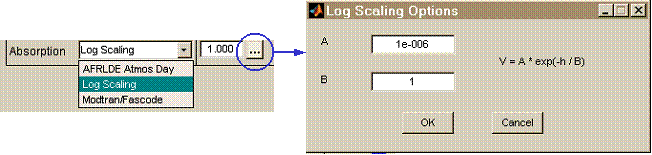
The three types of profiles are AFRLDE Atmos Day , Log Scaling and Modtran/Fascode . There are several options available within the classes: these options are accessed and set by pressing the "..." button to the right of the profile field. The right-hand panel of the illustration shows the options for the "Log Scaling" profile type.

AFRLDE Atmos Day: This profile, constructed by directed-energy (DE) researchers at the Air Force Research Lab, is defined for only two of the predefined wavelengths in the pull-down list of the wavelength input field: (a) the Nd:YAG wavelength 1.064mm, and the COIL (chemical oxygen-iodine laser) wavelength 1.31521mm (select 1.315mm in the pull-down list). This profile class has no options.

Log Scaling: This profile allows the user to specify a simple exponential altitude dependence, with a single scale height, of the form

The values of A (units of 1/m) and B (units of m) are specified by the user after pressing the "..." option button, and h is the altitude above ground level. This profile class allows the user to specify a simple, generic coefficient profile at any wavelength.

Modtran/Fascode: The code suite comprising MODTRAN and FASCODE has been developed over decades at the Air Force Geophysics Laboratory (a unit of the Air Force Research Laboratory), and represents the state of the art in computer modeling of atmospheric transmission and radiance. TurbTool includes a fairly extensive set of lookup tables derived from MODTRAN/FASCODE runs, that allow scattering and absorption profiles to be obtained quickly. The output set of FASCODE is deficient in the sense that scattering and absorption coefficients are not provided directly, even though internally the code uses the separate values. Therefore, part of the effort in constructing the lookup tables was to use a special procedure that involved code runs of MODTRAN and FASCODE with several different input options, in order to obtain outputs that allowed the separation of total attenuation into absorption and scattering coefficients. The look-up tables cover altitudes below 50 km.

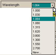The limitation of the lookup tables is that they are only valid for predetermined wavelengths, namely those listed in the pull-down list of the wavelength input field, as shown at right. This list includes several important high-power laser wavelengths: 1.030 mm = Yb:YAG, 1.064 mm = Nd:YAG, 1.315 mm = close to but not exactly the COIL wavelength of 1.31521 mm, 2.700 mm = neighborhood of HF (hydrogen-fluoride), 3.800 = neighborhood of DF (deuterium fluoride). Note that for purposes of thermal blooming in atmospheric propagation, only laser devices with high average total beam power are usually of interest. On the other hand, for purposes of simple transmission calculations, it would still be useful to treat arbitrary wavelengths. As explained in the discussion of the wavelength input field, the user has the option of requesting TurbTool to calculate new look-up tables at a custom wavelength. But, since that calculation can be time-consuming, the user also has the option to turn off scattering and absorption at a custom wavelength.

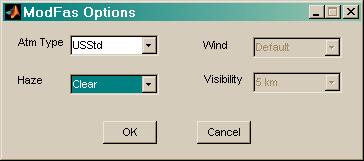Modtran/Fascode options can be specified by the user after selecting the profile and pressing the "..." option button. The options dialog box, shown at right, has four option fields: Atm(osphere) Type , Haze , Wind and Visibility . For full definitions of these options, the user must consult Modtran/Fascode documentation, but the general meaning should be fairly intuitive. Atm Type specifies the molecular atmosphere, and Haze specifies the aerosol. Wind and Visibility options will only be available for certain Haze selections.

5.3.1 Custom scattering and absorption profiles

As in the case of turbulence and wind distributions, completely custom scattering and absorption distributions may be defined by using the menu option View - Phase screen list to open a subsidiary window that contains an editable table of phase screen properties. The absorption and scattering coefficient values may be viewed in the table, or they may be plotted by using the menu command View - Scattering/Absorption Distribution .

5.4 Temperature profiles

The specification of temperature profile has no effect on any TurbTool calculations. The temperature profile is only used if TurbTool data is transferred to a WaveTrain runset that includes thermal blooming simulation.

6 Main screen inputs: Phase screens, Integration methods, and miscellaneous parameters

6.1 Miscellaneous parameters

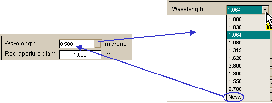
Optical wavelength: To specify the optical wavelength, the user must initially pull down a drop-down list of options, by clicking on the arrowhead at the right of the wavelength list box. This list contains a discrete set of wavelengths, plus the option New . New allows the user to specify an arbitrary wavelength (like the 0.500 mm illustrated above), but there is a complication. The listed discrete wavelengths have internal, pre-computed look-up tables of absorption and scattering profiles derived from MODTRAN/FASCODE, which allows for fast TurbTool computation. If New wavelength is selected, a further dialog box appears. This box asks whether the user wants TurbTool to compute a new look-up table of absorption and scattering (for the new wavelength):

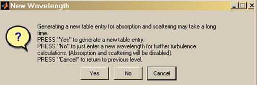
Computation of a new table can be a time-consuming operation, so we recommend to answer No unless the absorption and scattering coefficients will be needed for later WaveTrain thermal blooming calculations. Absorption and scattering coefficients have no effect on the turbulence calculations and turbulence screens generated by TurbTool. While the current TurbTool session is open, the new wavelength remains available in the drop-down list.

Rec(eiver) aperture diameter: This input parameter affects only one output item in the TurbTool screen, namely the Tyler tilt-tracking frequency, f_T, in the output table of integrated turbulence quantities.

6.2 Phase screens

TurbTool s phase screen definitions have two purposes. One purpose is to generate screen specifications that can later be transferred to WaveTrain for wave-optics simulation runs. A second purpose is to define screens that form the basis for the discrete integration method of generating integrated turbulence quantities.

The phase screen specifications are based on the following principles:
(a) The input # Phase Screens specifies the number of contiguous segments into which the propagation path is divided. Each of these segments will be represented by a phase screen.
(b) Two built-in options are provided for segment distribution:
     (b1) If input Screen Distribution is set to Equal Distance , then the propagation path is segmented into equal-length segments.
     (b2) If input Screen Distribution is set to Equal Strength , then the propagation path is segmented so that each segment has the same integrated C_n² value.
(c) Finally, three built-in options are provided for screen placement within their respective path segments:
     (c1) If input Screen Placement is set to Mid-point , then the screen positions are the segment midpoints.
     (c2) If input Screen Placement is set to Platform Side , then the screen positions are at the segment ends closest to the platform (recall that platform simply means z=0 in TurbTool-WaveTrain nomenclature).
     (c3) If input Screen Placement is set to Target Side , then the screen positions are at the segment ends closest to the target (recall that target simply means z=SlantRange in TurbTool-WaveTrain nomenclature).

The screens plot located immediately above the phase screens input block graphically reflects all the specifications discussed in the previous paragraph. The following figure shows two examples:

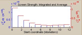
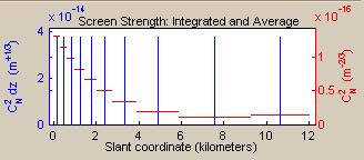
The path geometry for each example is the default geometry upon opening TurbTool, the turbulence profile is HV5/7, and # Phase Screens is set to 10. In the left-hand example, Screen Distribution is set to Equal Distance , and Screen Placement is set to Platform Side . The red horizontal bars indicate the path segments, and the height of these bars relative to the right-axis scale give the segment-average C_n² value. The blue vertical bars show the screen z-coordinates. In the right-hand example, Screen Distribution is set to Equal Strength , and Screen Placement is set to Mid-point . In this case, the segment-integrated C_n² value is, by construction, the same for all the screens.

In all cases, the segment-average C_n² value is the segment-integrated value divided by the segment length. Notice that this method of defining the screen strengths gives the discrete screen representation exactly the same total-path-integrated C_n² value as the continuum profile. This will be true no matter what location is specified for the screens within the segments. Therefore, at least the most fundamental path-integrated turbulence quantity, the simple integral of C_n², is faithfully represented by the discrete screen numerical model.

The final pair of screen input options, which are grayed out in the illustration at right, allow the user to define screens for a restricted sub-interval within the propagation path interval. That is, if the user clicks the check boxes to activate these fields, and then enters numbers such that
0 < (Begin turb at SR) < (End turb at SR) < SlantRange
then only the restricted interval will be segmented, and screens will be constructed for only those segments. However, the optical propagation path is still defined to start at z=0 and end at z=SlantRange: this latter fact impacts the calculation of the integrated turbulence quantities.

6.3 Integration methods

The final input in the screens input block, Integration method , controls the method of calculation for results that appear in the output table of integrated turbulence quantities. TurbTool provides two choices of integration method, Continuous and Discrete . The significance of the integration method is discussed in the document section on integrated turbulence quantities.

7 Main screen outputs: Table of integrated turbulence quantities

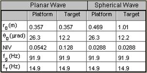Given the current propagation geometry, turbulence and wind profiles, wavelength and receiver diameter, and possibly the discrete screen specifications, TurbTool automatically calculates five key measures of the effects of turbulence. These are
(a) Fried s wave coherence length, r₀
(b) Isoplanatic angle, q ₀
(c) Normalized irradiance variance (NIV; sometimes called scintillation index)
(d) Greenwood frequency, f_G
(e) Tyler tilt-tracking frequency, f_T
The values of these five quantities are reported in the output table of integrated turbulence quantities, illustrated at right. The calculations are done for four cases:
(1) Plane-wave source, receiver at Platform (z = 0)
(2) Plane-wave source, receiver at Target (z = SlantRange)
(3) Spherical-wave source, receiver at Platform (z = 0)
(4) Spherical-wave source, receiver at Target (z = SlantRange)

The main restriction on validity of these results is that all are obtained from formulas derived using Rytov- or geometric-theory approximations. So, generally speaking, the results are only valid for weak to intermediate levels of integrated turbulence. The Greenwood- and Tyler-frequency formulas contain some additional approximations, which can result in significant deviations (say a factor of 2 or more) in practical cases of interest. The formulas that define the TurbTool integrated turbulence quantities are listed in a later section of the Guide. Because of the validity restrictions, corresponding results from a WaveTrain simulation run should not always match the TurbTool results. However, the TurbTool table can quickly provide a valuable guideline as to what to expect, and can indicate the turbulence regime in which the user is operating.

7.1 Integration method

The fundamental integrated turbulence formulas all have the general form

where A is a factor that may depend on wavelength, L is the slant range, z is the slant coordinate along the propagation path, w(z) is a path weighting function, C_n² and v(z) are the turbulence-strength and pseudo-wind profiles, and p is a constant exponent.

In the phase screens input block, the user selects Integration method = Continuous or Discrete . Integration method = Continuous means that Q is evaluated by numerical integration on a dense mesh, such that a close approximation is obtained to the continuum-space integral. In this case, the specifications of the discrete phase screens have no effect on the computation of Q.

Integration method = Discrete means that Q is evaluated using the discrete screen positions and screen C_n² values, according to the formula

where z_k are the screen positions, and Dz_k are the segment lengths (sometimes called screen thicknesses ). Generally, Q_discrete is not equal to Q. The one exception is the plain integrated C_n², because the screen C_n,k² values (i.e., the segment-average C_n²) were explicitly constructed to preserve this equality. Unfortunately, the equality between Q_discrete and Q can only be preserved for one weighting function, and we have chosen the unit weight function. Q_discrete does corresponds exactly to replacing the continuum profile by a comb-like profile whose component delta functions have strengths (C_n,k² * Dz_k). Therefore, within the limits of a Rytov formula, a wave-optics simulation result should give exactly Q_discrete. In this sense, TurbTool can be used to investigate the effects of the discrete screen model on key integrated turbulence quantities, without doing any wave-optics simulation runs. Specifically, one could investigate the effects of different segmentation choices (number of screens and distribution), and different placement of the screens within the segments.

7.2 Integration, screens, and top of the turbulent atmosphere

We have mentioned previously that TurbTool defines a top of the turbulent atmosphere by cutting off (setting to exactly 0) all C_n² profiles at altitudes higher than 50 km above MSL. (The user can change this boundary value by modifying a configuration file.) Some named profiles may already be defined as strictly zero for lower altitudes than 50 km, but that is dependent on the particular profile definition. The general top-of-turbulent-atmosphere cutoff that we are discussing now is additionally imposed on all profiles, and has the following motivation and consequences.

Despite the turbulence cutoff, propagation paths are allowed to have arbitrary portions above the turbulence cutoff (see the example in plot panel (B) in a previous section). The motivation for the cutoff is as follows. Given arbitrary possible path segments where turbulence is negligible, and given turbulence profiles that can change over several orders of magnitude along the propagation path, it is difficult for a single general-purpose numerical integration routine to guarantee acceptable accuracy for all possible situations. However, by defining a limited region that can contribute to any Q integral, we can use a simple but completely robust integration method (Simpson rule with a fixed, small step size) to guarantee good accuracy, say at least two significant figures, no matter how long the total propagation path is. The preceding discussion applies specifically to the calculation of the table of integrated turbulence quantities by the Continuous integration method.

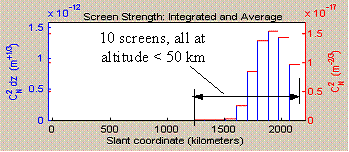The other implication of defining a top of the turbulent atmosphere concerns phase screen generation. If a propagation path has portions (one or two) above the top of the turbulent atmosphere, then only the path interval that lies below the top of the atmosphere will be segmented and have phase screens assigned. This will be evident when inspecting the plot of screen strengths and positions. In a previous section, the example in plot panel (B) defined a path with platform (z = 0) far above the top of the turbulent atmosphere, and then we specified # Phase Screens = 10, Screen Distribution = Equal Distance , and Screen Placement = Platform Side . The resulting screen layout is shown in the plot at right. It is clear that TurbTool has assigned all screens to a sub-interval of the full propagation path.

Note that if C_n² is set to strictly zero in a sub-interval to allow the restriction of the numerical integration domain of Q, the zero-turbulence sub-interval still affects some integrated turbulence quantities because the path weighting function in Q is cognizant of the propagation endpoints.

8 Main screen outputs: Miscellaneous

Min Path Alt above Ground : For the specified ground altitude and propagation path geometry, this output field shows the minimum altitude above ground level along the propagation path. Recall that TurbTool assumes a spherical-earth geometry, and that the ground altitude is uniform under the entire propagation path. This output field is located just above the table of integrated turbulence quantities.

Status : This output block, located at the bottom of the main GUI window, displays miscellaneous error and status messages.

Info : This output block, located at the bottom of the main GUI window, displays miscellaneous informational messages. For example, the Info block displays the model ground altitudes associated with standard turbulence profiles.

Optical transmission factors, t_X: optical transmission factors (0 £t £1) for the full propagation path, as determined from the screen absorption and scattering coefficients and segment lengths (screen thicknesses). t_scat is the transmission due to atmospheric scattering alone, t_abs is the transmission due to atmospheric absorption alone, and t_net is the net transmission. In each case, molecular and aerosol contributions are present, corresponding to the models discussed in the section on scattering and absorption profiles. These profiles will determine the thermal blooming if the atmospheric description is later used for a WaveTrain simulation run that invokes blooming. If absorption and scattering profiles have been disabled for a New wavelength, the transmission results are also disabled. The absorption and scattering settings have no effect on TurbTool s turbulence calculations.

9 Menus

The main TurbTool GUI window offers four pull-down menus. Help - Online help opens the present document. Key functions on the other menus are as follows.

9.1 File menu

The two key functions are:

Save as : This creates a file (in *.mat Matlab format) containing data that can be read by one of WaveTrain s AcsAtmSpec "constructors" to specify the turbulent atmosphere for a WaveTrain system and runset. Specifications that can be transferred in this way include the screen positions, segment thicknesses and C_n² values, the true-wind speeds associated with each screen, and the inner and outer scale values. In brief, all the discrete data that appears in the Phase Screens Table can be transferred as a unit in this way from TurbTool to WaveTrain.

REMARKS ON DATA TRANSFER FROM TurbTool TO WAVETRAIN:

To accomplish the data transfer using TurbTool's save file, the AcsAtmSpec constructor syntax needed in the WaveTrain run set is "AcsAtmSpec(filename, Cn2factor)", where "filename" is the *.mat file created by TurbTool, and "Cn2factor" is yet another overall multiplier that may be applied within WaveTrain. See the WaveTrain User Guide for further details on AcsAtmSpec usage.

As an alternative to the data file transfer procedure, users may prefer to manually copy TurbTool-generated data into AcsAtmSpec in a WaveTrain run set. This would involve the use of other allowed forms of the AcsAtmSpec constructor arguments, where various vectors such as screen positions and C_n² values are explicitly entered. While the manual procedure may involve a little more labor, some users may find that it provides a greater sense of user control and later readability of the runset. In any case, this is the most flexible way of using TurbTool-generated data as WaveTrain input.

CAUTION: there is one limitation on the completeness with which atmospheric specification data can be transferred from TurbTool to WaveTrain: the TurbTool platform and target velocities are not readable by WaveTrain. This situation exists because these velocity specifications are not part of WaveTrain s atmospheric modules, but rather are specified separately in WaveTrain by using TransverseVelocity modules. The practical significance of this is that the user who wishes to transfer TurbTool specifications to a WaveTrain runset must manually enter the appropriate platform and target velocity specifications in WaveTrain's TransverseVelocity modules. (In contrast to this, values of the true atmospheric wind, specified via the wind profile options, are attached directly to the phase screens specifications, and these true-wind velocities will automatically be transferred to the WaveTrain atmospheric blocks when the constructor syntax "AcsAtmSpec(filename,Cn2factor)" is used.)

If the user wishes to transfer TurbTool save-file data into a WaveTrain system that includes thermal blooming, then WaveTrain's MtbAtmSpec constructor must be used. The extra relevant data now consists of the discrete absorption, scattering and temperature profiles. To accomplish the data transfer, the required constructor syntax in WaveTrain is "MtbAtmSpec(filename, propnxy, propdxy)", where "filename" is the *.mat file created by TurbTool, and "propnxy" and "propdxy" are the propagation mesh dimension and physical spacing. See the WaveTrain User Guide for further details on MtbAtmSpec usage.

Load : This allows the TurbTool user to load back into TurbTool a *.mat file that was previously saved using the "Save as " option.

9.2 View menu

The View menu provides several types of functions.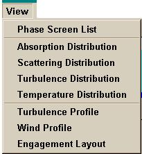

View - Phase Screen List brings up a subsidiary window that contains an editable table of phase screen properties.

View - Xxx Distribution creates a new plot window showing one of the following discrete distributions: absorption, scattering, turbulence, or temperature. In the case of turbulence, this plot is identical to the Screen Strength plot that appears on the main GUI screen. The only difference is that the View -generated window is a separate, editable Matlab plot window. Users may find this convenient for further work or documentation purposes.

View - Turbulence Profile creates a new plot window showing the continuous turbulence profile that was selected in the main-screen input block entitled Profiles . The overall strength scale factor specified by the user is included in the plotted profile.
The phase screens whose strengths are plotted in the Screen Strength plot are derived from this underlying continuous profile and the specified path segmentation, as defined elsewhere. The new plot window is an editable Matlab plot window.

View - Wind Profile creates a new plot window showing the continuous wind profile that was selected in the main-screen input block entitled Profiles . The plotted wind profile is the magnitude of the wind speed, including the overall x and y scale factors specified by the user. The profile shows only the true atmospheric wind, not the pseudo-wind that includes target and platform velocity effects.

View - Engagement Layout creates a new plot window showing the same engagement geometry plot that appears on the main GUI screen. The only difference is that the View -generated window is a separate, editable Matlab plot window. Users may find this convenient for further work or documentation purposes.

9.3 Tools menu

The options in the Tools menu allow the user to return certain data structures to the Matlab workspace from which TurbTool was opened. The data in question is thus made available for further custom manipulation by the user.

Make ATMStruc : Stores the TurbTool-defined data in a Matlab structure that has the form of the ATMStruc data structure used in a separate code suite called ATMTools. The purpose of this option is to facilitate future interoperability or merger of TurbTool and ATMTools.

Make TurbTool Struc : Stores the TurbTool-defined data in a Matlab data structure native to TurbTool.

10 Phase screens list (table)

A table that lists all details of the phase screens can be opened by the menu action View - Phase Screen List . A sample table, for a case where # Phase Screens = 5, is shown below. This table lists all parameters of the phase screens that were defined in the main GUI window, and also contains some extra parameters that are not settable from the main window. Some columns of this table are editable, thereby allowing the user to define a completely custom set of phase screens.

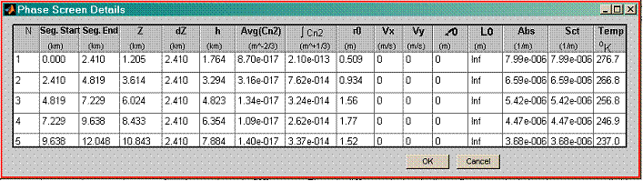
The table contains one row for every propagation path segment, or equivalently for every screen. Each column refers to a different property of that segment or screen. The principles used in the path segmentation and screen generation were discussed in a previous section. Physical units are specified in the table header for all quantities.

10.1 Editable columns

A subset of the table columns are editable. When manual edits are entered into the table, dependent table columns update immediately. An exception to the immediate-update rule occurs if the user enters some temporarily inconsistent data (such as overlapping segment boundaries) in the course of making more extensive changes. In that case a status warning appears until the user enters further edits that make the table numbers consistent again. Upon returning to the main TurbTool window, other updates may occur in the main window settings and outputs.

To begin editing a field, double-click in the desired field. The following columns in the table are editable:

Seg. Start, Seg. End, and Z: These are, respectively, the start and end z coordinates of the path segments, and the z coordinates of the screen locations.

AvgCn2: Segment-average C_n² value. Manually editing this column, and the preceding coordinates columns, allows the user to specify a completely custom turbulence profile.

Vx, Vy: Wind velocity components assigned to screens. Note that this refers only to the true atmospheric wind, not the effective (or pseudo-) wind that includes the platform and target velocities. The velocity values assigned to a screen are the average values of the continuous wind profile over the propagation segment corresponding to the screen. This is consistent with the manner in which the screen-C_n² (AvgCn2 in the table) is defined.

l0, L0: Inner scale and outer scale lengths associated with the screens. These settings have no effect within TurbTool: the formulas used to compute integrated turbulence quantities within TurbTool all assume the default values of zero inner scale and infinite outer scale. However, if finite inner and outer scale values are transferred to WaveTrain, the screen-generator routines in WaveTrain do respond to these specifications.

Abs, Sct: Atmospheric absorption and scattering coefficients, m. These coefficients determine the optical transmission factors listed in the main GUI window. The key relation is that intensity transmission for a single segment k is given by

where X represents abs, scat, or net, and where m_net = m_abs + m_scat.

Temp: Atmospheric temperature distribution along the propagation path. This is not used by any TurbTool calculations. If the data is transferred to WaveTrain, the temperature distribution is used in setting up thermal blooming screens, if the WaveTrain model invokes thermal blooming.

10.2 Non-editable columns

dZ: Length of segment (referred to sometimes as the thickness of the phase screen)

h: Height above mean sea level corresponding to Z of screen

òCn2: Path-integrated C_n² for segment. Upon opening the table, this is the segment-integrated C_n² value obtained from the continuous profile that was specified in the Profiles block of the main TurbTool window. But, if a manual edit is made in the AvgCn2 column of the table, then òCn2 is simply reset to AvgCn2*DZ.

r0: In the mechanics of generating phase screen realizations for wave-optics simulation, screen strengths are often specified in terms of a screen r0 , instead of by the equivalent (AvgCn2, dZ) or òCn2. The r0 in question is a plane-wave r0 for propagation through the path segment modeled by the screen.

10.3 Main-screen updates upon return from Phase Screens table

The main TurbTool window is locked while the Phase Screens Details table is open. To return to the main window, the user has the two table options Cancel and OK .

Pressing Cancel will cancel any edits that were made in the table, and return the user to the main TurbTool window in the same state as before the Phase Screens table was opened.

Pressing OK will return the user to the main TurbTool window, and may cause several changes to occur in the main window outputs and settings. The changes in the main window are as follows:
(a) If the user edits the fields Seg. Start , Seg. End , or Z , then Screen Distribution and Screen Placement are changed to User Spec .
(b) If the user edits the field AvgCn2 , then the field Integration Method is changed to Discrete , since the previously selected continuous C_n² profile is no longer meaningful.
(c) If the user edits the field "AvgCn2", then the Turbulence Profile selection is changed to "User Spec", since the previously selected continuous C_n² profile is no longer meaningful.
(d) In analogy with rule (c), if the user edits the fields "Vx", "Vy", "Abs", "Sct", or "Temp", then the corresponding Profile selections are changed to "User Spec".

Pressing OK in the Phase screens table will also cause values in the output table of integrated turbulence quantities to update in accordance with any of the changes described just above.

11 Configuration file settings

TurbTool uses a short configuration file to establish a few basic numerical settings. The file is named GetConstants.m , and is located in the top-level TurbTool directory. In normal operation, the user does not interact directly with this file. However, at some point the user might wish to manually edit this file (using any text editor) to adjust certain settings. As an example, the user may want to adjust the top of turbulent atmosphere setting to something other than the default 50 km AMSL altitude.

12 Formulas used by TurbTool for integrated-turbulence quantities

The formulas encoded in TurbTool are derived using Rytov- or geometric-theory approximations to turbulent propagation. So, generally speaking, the results are only valid for weak to intermediate levels of integrated turbulence. The Greenwood- and Tyler-frequency formulas contain some additional approximations regarding system bandwidths, which can result in significant deviations (say a factor of 2 or more) in practical cases of interest. Because of these validity restrictions, corresponding results from a WaveTrain simulation run should not always match the TurbTool results.

The formulas in this section assume a coordinate system where the z-axis is the nominal propagation direction, the source plane is at z = 0, the receiver plane is at z = L, and the turbulence profile is given by C_n²(z). There are two canonical cases for which analytical results are commonly given, the spherical-wave case and the plane-wave case. The spherical-wave formulas apply when z = 0 designates the position of a point source. The plane-wave formulas apply when we assume that a plane wave is the initial condition at z = 0. Note that in the spherical-wave case, a particular choice of C_n²(z) may place the point source far outside the region of non-0 turbulence: in that case the spherical-wave numerical results will approach the plane-wave results.

CAUTION: Integrated turbulence quantities reported in the output table are the results of high-density numerical integration of the formulas below, IF AND ONLY IF the GUI option Integration method = Continuous is selected. If the GUI option Integration method = Discrete is selected, then a coarser sum is computed based on the phase screen positions and screen-C_n² values that have been defined. This distinction was previously discussed in the section on integration methods.

Fried s wave coherence length:

The transverse coherence length r₀ is a measure of how far apart two points must be (transverse to the propagation direction) before the rms wavefront difference due to turbulence exceeds a critical value. The results reported by TurbTool are as follows:

Plane-wave case:

Spherical-wave case:

Normalized irradiance variance (NIV):

If I is the irradiance (W/m²) at a point, then the usual measure of turbulent irradiance fluctuation is the normalized irradiance variance (NIV). NIV is the variance of I at a point divided by the square of the mean I at that point. Equivalently, if we consider the normalized irradiance J = I /(mean I) , then NIV is simply the variance of J. In the lowest-order Rytov approximation, theoretical results are actually obtained for a closely-related quantity, namely the variance of the log-amplitude, often denoted by s _c² in theoretical references. For weak to moderate turbulence, i.e., prior to the onset of saturation, the relation NIV = 4 s _c² is a good approximation. Using this approximation, the first-order Rytov results reported by TurbTool are as follows:

Plane-wave case:

Spherical-wave case:

Isoplanatic angle:

The formula for isoplanatic angle q₀ is the same for plane- and spherical-wave cases:

(Note: as stated in the introductory paragraphs, the directional conventions for these formulas are that the source plane is at z = 0 and the receiver plane is at z = L. That is, the vertex of the isoplanatic angle referred to by the formula is at z = L.)

Greenwood and Tyler frequencies:

The Greenwood and Tyler frequencies, f_G and f_T respectively, refer to feedback control system bandwidths required to achieve a certain performance level in rejecting atmospheric disturbances. The Greenwood frequency refers to a composite of all disturbance spatial frequencies, while the Tyler frequency refers to the tilt component only. The same formulas hold for plane- and spherical-wave cases:

where is the magnitude of the effective or pseudo-wind transverse velocity at coordinate z. The vector pseudo-wind velocity may have arbitrary x and y components, but only the magnitude enters into the Greenwood and Tyler frequencies.

where D is the receiver aperture diameter over which the tilt is defined, and is again the magnitude of the effective or pseudo-wind transverse velocity at coordinate z .

13 Independent use of turbulence profile subroutines

Some users may find it useful to independently use the TurbTool subroutines that compute the standard vertical profiles of C_n². This would be easy to do, since each subroutine is a separate Matlab m-file. The routines are located in the subdirectory \turb under the main TurbTool directory. The routine names all have the form tp*.m : for example, the Clear-1 turbulence vertical profile is defined by "tpCL1N.m". Each file consists of a wrapper routine and a subroutine that actually defines the standard C_n² profile. Among other things, the wrapper routine handles the ground-altitude adjustment. The routines are sufficiently documented (and short enough) that any Matlab user will easily be able to run them independently.

14 Programming notes

TurbTool is a Matlab GUI application that consists of a suite of Matlab m-files. To assist in potential future modifications and extensions of TurbTool, we provide a flow-chart that shows the calling relationships among the key computational routines of the TurbTool code suite. The graphical elements of the GUI are constructed using the Matlab GUIDE environment.

For development comments and questions, contact:
Boris Venet MZA Associates Corp. 505-245-9970 venet@mza.com
Morris Maynard MZA Associates Corp. 937-684-4100 morris@mza.com