Copyright © 1995-2010 MZA Associates Corporation
WaveTrain User Guide
Steve C. Coy and Boris P. Venet
Revision information
Functional specifications in this User Guide cover WaveTrain versions up to ver. 2010A. Ver. 2010A is scheduled to be released in March 2010.
CAUTION: a few subsections of the User Guide may have illustrations in which older versions of the graphical user interfaces (GUIs) appear. In such cases, the GUI features and control layout will usually be similar enough to the current version so that no confusion arises; if the layout differences are critical to the subject matter of the subsection, some commentary will be given.
Last User Guide revision date: 5 Sep 2011.
*************************************************************************
WaveTrain is a code suite that provides computer modeling of optical propagation through the turbulent atmosphere, and the modeling of associated optical imaging, beam control and adaptive optics systems. WaveTrain provides a connect-the-blocks visual programming environment in which the user can assemble beam lines, control loops, and complete system models, including closed-loop adaptive optics (AO) systems. WaveTrain also provides graphical interfaces for setting up adaptive optics geometries and turbulence profiles, and a spreadsheet-style interface for setting up and executing parameter studies. The generated output, comprising imagery, complex-field quantities, control signals and the like, can be inspected in a WaveTrain viewer, or can be loaded into MatlabTM or other environments for further analysis and post processing.
This User Guide is designed to serve as a tutorial introduction to WaveTrain for new users, and a reference for more experienced users. The User Guide attempts to be as comprehensive as possible in documenting the scope, usage rules, and assumptions of the WaveTrain code. In doing so, we may occasionally digress into short tutorials on topics in optical propagation theory and adaptive optics, but for detailed theory background we refer the reader to the standard literature. WaveTrain is a complex code, and its pieces have been constructed and assembled by numerous contributors at MZA Associates (and some contributors elsewhere). Generation of documentation is an ongoing effort, and the elements of WaveTrain are not all documented at the same level of detail. When users have questions regarding WaveTrain, we ask them to proceed as follows. First, search the present User Guide, the MZA web-site update material, the index to all WaveTrain documents, and the individual module documentation in the WaveTrain Components and Effects Library. If this fails to resolve the question, feel free to contact MZA by email or phone.
WaveTrain is built atop tempus, a general-purpose simulation tool also created by MZA Associates. tempus provides the visual programming environment, the software architecture, and all the basic mechanisms that support model-building and simulation. WaveTrain adds a component library for modeling optical systems and effects, and several application-specific GUI components. The latter comprise a tool for setting up wavefront sensor and deformable mirror geometries, a tool for specifying turbulence distribution along an optical propagation path, and a tool for setting up and executing parameter studies. The GUI tool for wavefront-sensor and DM configuration also has associated Matlab routines for a variety of AO tasks, such as computing reconstructor matrices. The GUI tool for specifying turbulence distributions also performs a variety of useful calculations of integrated turbulence quantities based on theoretical formulas; these can be used as a starting point for initially estimating or bounding answers to be obtained from the wave-optics simulation.
To get a quick idea of what WaveTrain can do and how one can use it, start with our quick tour (this should take less than 10 minutes).
For a more detailed introduction (a few hours), work through one or
more of our step-by-step tutorials, particularly the Guide
section on Assembling and running a WaveTrain
model - Tutorial. After these introductory exercises, there will
undoubtedly still be many details that are fuzzy to the new user. We
suggest that the best procedure at that
point is:
(a) skim the rest of this User Guide to get a sense of the organization
and contents;
(b) attempt construction of original simple systems, based on what you
have learned from the "Assembling" section and auxiliary
tutorials;
(c) as conceptual and procedural questions then arise, dive into the
remaining detailed documentation chapters of this User Guide as needed.
By way of preview, we mention the following details
chapters:
(*) For physics-oriented issues and usage details regarding important
specific WaveTrain library systems, users should consult the chapter
Modeling details.
(*) For details regarding data entry in the two editor windows, users
should consult the chapter Data entry in subsystem
parameters and inputs, and in the Run Set Editor.
(*) For details regarding TrfView, trf files (recorded outputs) and the
extraction of trf
data, users should consult the chapter Inspecting and
post-processing WaveTrain output: *.trf files, TrfView, and Matlab.
(*) For details regarding the construction of user-defined WaveTrain
subsystems, users should consult the chapter
Creating user-defined WaveTrain components.
WaveTrain documentation and updates on the Web
Improvement of the WaveTrain documentation is an ongoing
project. For the most recent version of the WaveTrain User Guide and
allied documentation, the user should refer to MZA's web site:
http://www.mza.com/Default.aspx#productstab-wtdocs,
then click on "WaveTrain User Guide" under the Index.
Here the
user will always find the most recent version of the User Guide, as well as
material that has not yet found its way into the general Guide. The latter
material may include auxiliary
documentation on special topics, extra tutorials not accessible through the User
Guide, and WaveTrain bug notes, discussions, and patches.
In addition, some auxiliary documentation relevant to WaveTrain may be found
under the "tempus" heading at MZA's web site: for a list of those documents,
see:
http://www.mza.com/Default.aspx#productstab-tempus.
Index to all WaveTrain Documents
J. Goodman, Statistical Optics, Ch. 8, Wiley-Interscience, 1985
V. Tatarski, Wave Propagation in a Turbulent Medium, McGraw-Hill, New York, 1961
A. Ishimaru, Wave Propagation and Scattering in Random Media, Chs. 16-20, IEEE Press/Oxford U. Press, reissued 1997 (original pub. Academic Press, 1978)
R. Tyson, Principles of Adaptive Optics, Academic Press, New York, 1991
M.C. Roggeman and B. Welsh, Imaging through Turbulence, CRC Press, 1996.
J. Hardy, Adaptive Optics for Astronomical Telescopes, Oxford University Press, 1998
L. C. Andrews and R.L. Phillips, Laser Beam Propagation through Random Media, SPIE Optical Engineering Press, 1998.
R.E. Hufnagel, "Propagation through Atmospheric Turbulence", in The Infrared Handbook, Ch. 6, Environmental Research Institute of Michigan and Office of Naval Research, rev. ed., 1985.
R.R. Beland, "Propagation through Atmospheric Optical Turbulence", in Atmospheric Propagation of Radiation, vol. 2 of The Infrared and Electro-Optical Systems Handbook, SPIE Press, 1993.
User Guide Contents
WaveTrain documentation and updates on the web
Index to all WaveTrain documents
WaveTrain step-by-step tutorials
Assembling and running a WaveTrain model - Tutorial
Create a new WaveTrain system model
The WaveTrain component libraries
Copy components from one System Editor window to another
Saving systems, opening existing systems
Component parameters, inputs, and outputs
Display/hide graphical elements
Create a new run set for the WaveTrain system
Further WaveTrain details - next steps
Connecting WaveTrain components
Physical units and nomenclature
Spatial coordinates and direction nomenclature
Modeling of optical systems in "object space"
Sign and phasor conventions for tilt, focus and general OPD
Sensor timing, CW sources and pulsed sources
Transverse (x,y) displacement and motion (TransverseVelocity and Slew)
Transverse displacement and size of propagation mesh
Transverse displacement and size of phase screens
Longitudinal (z) displacement and motion
Optical propagators in WaveTrain
Choosing mesh settings for optical propagation
Setting up Fresnel propagations
Using the PropagationController
Using atmospheric turbulence models
Atmospheric modeling using TurbTool or PropConfig
Using atmospheric thermal blooming models
Basic sensor modules: TargetBoard, SimpleFieldSensor and Camera
Spatially integrating WaveTrain sensor outputs
Interference of polychromatic fields
Splitting and combining optical paths
Using Polarizers to separate light from different sources
Adaptive optics models (wavefront sensors, deformable mirrors, tilt trackers)
Optically-rough reflectors, and modeling of speckle
Components for data-type conversion
How to use spatial filters and absorbing boundaries
Using WaveHolder to avoid performing redundant propagations
Data entry in subsystem parameters and inputs, and in the Run Set Editor
C-language syntax for expressions and basic math functions
Procedures for entering vectors, arrays and "Grids"
Procedures for modifying vectors, arrays, and "Grids"
The functions "gwoom" and "GridGeometry"
Miscellaneous special functions and operators
Status bulbs and status checking
Miscellaneous rules and tips for Run Set and System Editors
Inspecting and post-processing WaveTrain output: *. trf files, TrfView, and Matlab
Loading trf data into Matlab without TrfView
Key commands for working with trf data in Matlab
Creating user-defined WaveTrain components
Creating a new component by composing existing library modules
Creating a new atomic component from a Matlab m-file (m-system)
Creating a new atomic component - general
How WaveTrain works at the source code level
WaveTrain "starter systems" for constructing new atomic systems
Using WaveTrain models to gain understanding of the modeled systems
How to set up and execute parameter studies
Averaging over stochastic effects
A quick tour of WaveTrain
Modeling an optical propagation system in WaveTrain is
essentially a four-step process. The steps are:
(1) Assemble the WaveTrain model, by copying optical and processing
components from the WaveTrain component libraries, and
connecting the inputs and outputs of the components.
(2) Set the numerical parameters of all components, and the simulation
timing parameters.
(3) Run the simulation.
(4) Inspect the WaveTrain simulation outputs, and post-process as needed.
Steps (1)-(3), and parts of step (4), are carried out within WaveTrain's visual
programming environment. Arbitrary post-processing in step (4) requires
the use of an auxiliary visualization and computation environment, such as
Matlab™.
Step 1 - Assembling and connecting the WaveTrain components:
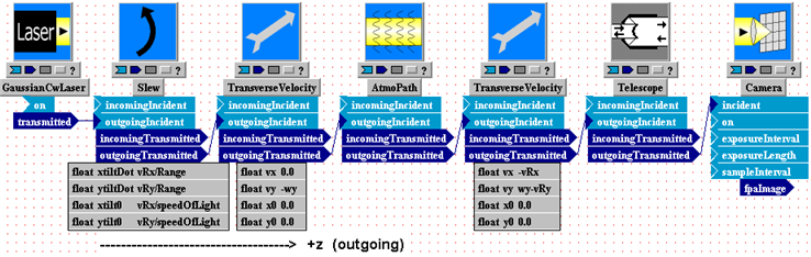
For example, suppose we want to look at the optical effects of propagation through atmospheric turbulence. We might assemble a basic model like that shown below:
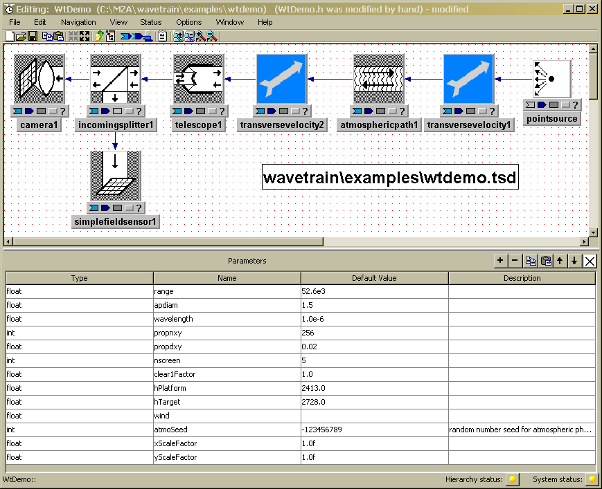
Figure: WaveTrain's System Editor, showing the WtDemo propagation model
The window in the above picture is called the System Editor window (equivalently, the Block Diagram Editor), and is used for assembling the optical model from library components. The present model consists of eight components (also called subsystems, or modules) connected together. All of the subsystems shown can be found in the WaveTrain component library, and all of the connections in this particular model represent optical interfaces. (Connections that correspond to electronic or general data signals are also available). Starting at the far right, we have a Point Source, a TransverseVelocity, an AtmoPath, another TransverseVelocity, a Telescope, and an IncomingSplitter, which splits the incoming light and sends part to a Camera and part to a SimpleFieldSensor. The PointSource represents an idealized point source, radiating uniformly in all directions. The two TransverseVelocities can be used to model source and detector transverse motion, and/or a true wind velocity. The AtmosphericPath module is a complex module that represents two processes: (a) the optical effects of turbulence using multiple discrete phase screens distributed along the propagation path, and (b) the diffractive propagation of light along the propagation path. By assigning screen motions, AtmosphericPath can also model transverse wind velocities that vary spatially along the propagation path. In between the phase screens the optical wavefronts are propagated using a two-step FFT propagator. The Telescope applies an aperture and a focus adjustment to the incoming light. The IncomingSplitter duplicates the incident beam and sends it out into two branches. The SimpleFieldSensor records the complex field - amplitude and phase - at the aperture plane. The.Camera brings the light to a focal plane (using a Discrete Fourier Transform) and records the intensity pattern in that focal plane.
This relatively simple model can be assembled by a novice user in an hour or so - see our step-by-step tutorials - and it is not a toy; it can do serious calculations.
Step 2 - Setting the numerical parameters of all components:
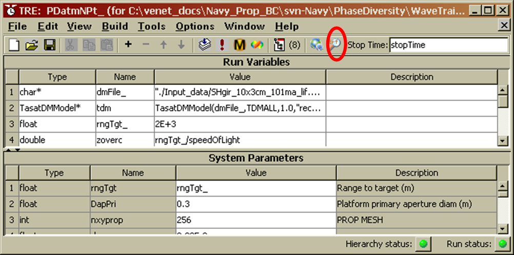
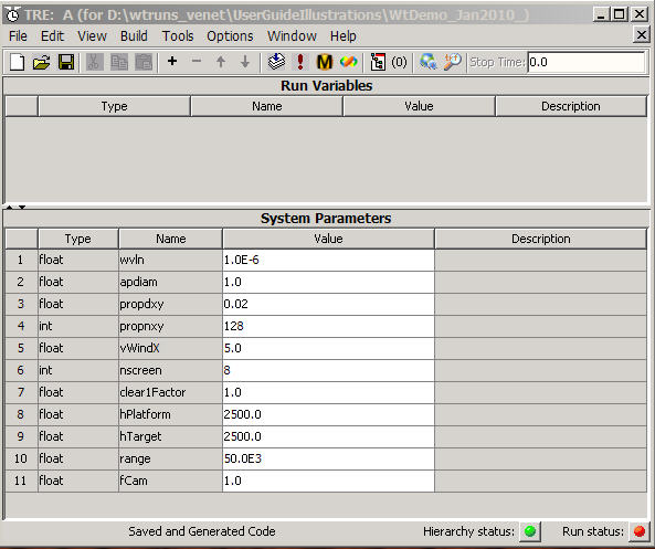
After assembling and connecting the system components, the user must assign all the necessary parameter values. These include source powers, aperture diameters, propagation distances, propagation mesh dimensions, turbulence phase screen parameters, sensor spatial and timing parameters, etc. Setting all these parameter values is done partly in the System Editor window illustrated above, and partly in a second editor window, called the Run Set Editor. A sample Run Set window for the preceding system is shown below (in the window title, "TRE" stands for the full name "tempus Run Set Editor"):
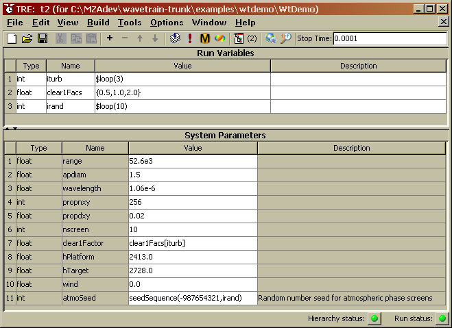
Figure: WaveTrain's Run Set Editor - a run set for the WtDemo propagation model
Step 3 - Running the simulation:
After specifying all the parameter values, the user initiates execution of the simulation with a few button clicks in the Run Set Editor. Upon completion of the execution, WaveTrain's output - a combination of sensor images, complex field data, and/or electrical signal data - is stored to data files in a form that can be conveniently accessed for visualization and post-processing.
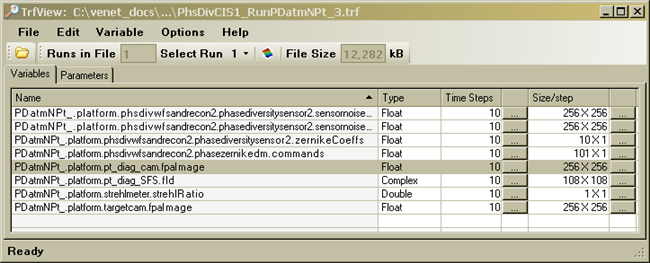
Step 4 - Inspecting and post-processing the WaveTrain outputs:
Visualization and limited post-processing of outputs can be accomplished using the TrfView viewer that is part of WaveTrain suite. Typical outputs might be the instantaneous wave amplitude and phase maps in the "telescope1" pupil plane of the above WtDemo model. These particular outputs are based on the complex optical field sensed by the "simplefieldsensor1" component in the model. Sample outputs as displayed in TrfView are shown in the following figure:
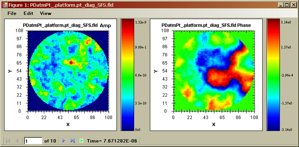
Figure: WaveTrain sample outputs - amplitude (left), and phase (right) maps in the telescope pupil of the WtDemo system, as displayed in WaveTrain's TrfView viewer
Completely general visualization and post-processing can be accomplished using Wavetrain's Matlab
™ interface. WaveTrain can be used with or without Matlab, but WaveTrain provides a full-featured Matlab interface. Not only can WaveTrain output data be conveniently imported into Matlab, but also complete WaveTrain system models can be created and executed from within Matlab, or converted into "S-functions" for use within Simulink, which is Matlab's general purpose simulation environment. Additionally, Matlab m-files can be automatically converted into WaveTrain components, so that Matlab users have a simple way of creating custom WaveTrain components to supplement the WaveTrain library.By varying the parameters of the WtDemo model illustrated in the above figures, the user can investigate a wide variety of issues fundamental to the problem of optical propagation through turbulence. These issues include the statistics characterizing the spatial and temporal variation of the amplitude and phase effects, in both pupil and image planes of a receiver, and the way those statistics changes when the distribution of turbulence along the path is changed.
Auxiliary tools for defining input parameter specifications:
In addition to the fundamental System Editor and Run Set Editor, the WaveTrain suite includes several other graphical user interfaces (GUIs). The purpose of these auxiliary tools is to assist in setting the numerical inputs of some of the WaveTrain components, particularly the more complicated modules that deal with atmospheric turbulence and adaptive-optics components. For example, there is a Matlab GUI for setting up deformable mirror and wavefront sensor geometries. Also, there is a Matlab GUI that facilitates turbulence strength and atmospheric specifications, and allows the evaluation of certain analytical formulas that estimate key integrated-turbulence quantities (such as scintillation variance and Fried's r0).
Scope and development of WaveTrain:
WaveTrain is designed to be useful to scientists, engineers, teachers, and students engaged in the design and development of advanced optical systems, or in the study of propagation through turbulence and associated adaptive optical systems. It is equally well-suited for simple models, like the example shown above, for intermediate complexity models such as are typically used in concept exploration, and for the kind of detailed engineering models necessary for accurate performance prediction, design refinement, and trouble-shooting. We are continually adding new components and features, and making improvements, often in response to customer feedback. If you need or want a feature that we don't yet offer, please let us know. Alternatively, WaveTrain is designed to be extensible, so you can create your own components to supplement the WaveTrain library, as described in creating your own WaveTrain components.
WaveTrain step-by-step tutorials
The User Guide chapter immediately following the present one provides an introductory tutorial to assembling and running WaveTrain models. That tutorial is a compromise between constructing the simplest possible first system, and constructing one that is still fairly simple yet will be physically interesting to most WaveTrain users. A new user can work through that tutorial in a few hours.
We also provide here several links to other tutorial briefings that have been
used by MZA personnel when leading WaveTrain training sessions or short courses.
Slight drawbacks of those documents may be that: (i) they may use some
illustrations or procedures from older versions of WaveTrain, resulting in
occasional confusion, (ii) since the briefings were meant to be used in a
trainer-led class, some explanatory sentences may be missing from the
briefing charts. Despite those warnings, users may still find the extra
tutorials useful. These tutorial briefings may be found on the
WaveTrain
documentation page on MZA's website. These extra tutorials are
accessible from the following links on that web page; roughly in order of
complexity, they are
(a) "WaveTrain
User's Quick Start"
(b) "WaveTrain Tutorial (March 2008)"
(c) "The Whiteley Tutorial model".
Note that the most recent version of the present WaveTrain User Guide may also be found on the same web page, at the link WaveTrain User's Guide.
WaveTrain Examples Library
After working through the introductory tutorial, and in conjunction with the construction of original WaveTrain systems, users may find it useful to inspect some of the example systems in the WaveTrain Examples Library. The examples library comprises WaveTrain systems and run sets which are delivered with WaveTrain. The purpose of the examples is to provide working systems which involve application of WaveTrain concepts and to give users a start on building more complex systems. The example systems are distributed with standard WaveTrain installations, and may be found in the subdirectory "wavetrain\examples\" of the WaveTrain installation directory. (Disclaimer: it should not be assumed that the examples provided there are fully valid for any particular user application).
Assembling and running a WaveTrain model - Tutorial
We suggest that new users begin their WaveTrain study by working through the
following tutorial. The tutorial has the following goals:
(a) To lead a new user step by step through the construction and
execution of a WaveTrain simulation.
(b) To introduce a new user to several of the key WaveTrain components
that are needed for most WaveTrain systems.
(c) To introduce the user to some of the specialized nomenclature that is
used in the WaveTrain program.
(d) To introduce the user to TrfView, which is WaveTrain's utility for
quick inspection and plotting of simulation results.
Create a new WaveTrain system model
To start the WaveTrain user interface, double-click the Wavetrain desktop
shortcut, or use the typical Windows menu sequence, 'Start - Programs - MZA
Associates Corp - WaveTrain'. The desktop shortcut and start group should
have been generated during the WaveTrain installation process.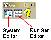
Starting WaveTrain as above simply brings up a small toolbar with the title "TVE". TVE stands for Tempus Visual Editor, which is the overall graphical interface program through which the user interacts with WaveTrain. A picture of the TVE toolbar is shown at right.
To begin the setup process for a new system, go to the TVE toolbar and left-click on the System Editor button. This brings up a blank System Editor window, as shown below:
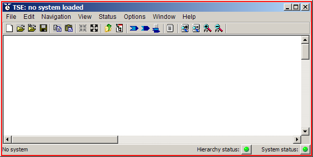
Figure: Blank System Editor window
--------------------
For WaveTrain Ver. 2010A and later:
In the File menu of the editor window, execute the sequence
File - New - New System.
This changes the window title to "NewSystem", instead of "no system loaded" as
shown in the above illustration. The window is now ready to accept the
insertion of components to build a new system.
--------------------
--------------------
For WaveTrain Ver. 2009A and earlier:
The blank Sytem Editor window opens already in the "NewSystem"
state, ready for insertion of components to build a new system.
--------------------
At this point, you are ready to begin creation of a WaveTrain system by copying the components you desire from the WaveTrain libraries into the NewSystem window. There are several methods for inserting library components into a new system:
(1) You can open a second System Editor window, and in that window open an iconic representation of the WaveTrain library. Then you can copy and paste individual components from the library into your new system. This is a good method for comprehensively browsing the available library systems, particularly when you are still unfamiliar with the library contents.
(2) It is
also possible to insert components by
(a) inserting them directly from a library directory
listing, or
(b) copying and pasting components or groups of
components from existing systems.
We will discus some of these alternate methods later in the present chapter.
In the remainder of this tutorial, you will use the basic method (1) to create a new system.
The WaveTrain component libraries
You will now insert components into a new system, using the basic Method (1) above.
--------------------
For WaveTrain Ver. 2010A and later:
(1) Start WaveTrain, and press the TVE toolbar System Editor button
(already done in the above subsection).
(2) In the File menu of the editor window, execute the sequence
File - Open - Master Library.
This causes a second, separate System Editor window to open, and after a few
seconds of loading time you will see a display of icons as in the following
screen snapshot. These icons comprise the WaveTrain "component libraries":
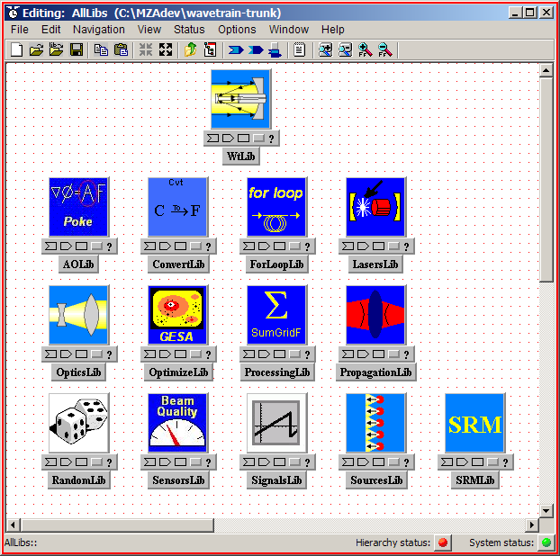
Figure: All the WaveTrain component libraries, in WaveTrain Ver. 2008 and later
(3) Now double-click on the icon labeled "
WtLib" (top row in the above figure). You will then see a set of six icons representing "sub-libraries", as shown in the following figure:
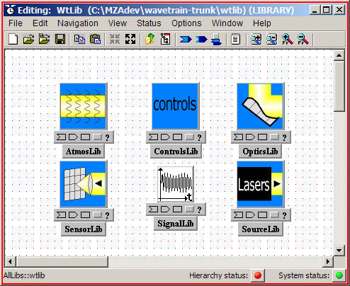
Figure: Contents of the WtLib library
--------------------
--------------------
For WaveTrain Ver. 2009A back to Ver. 2008:
(1) Start WaveTrain, and press the TVE toolbar System Editor button
(already done in the above subsection).
(2) Press the TVE toolbar System Editor button again to open a second System
Editor window.
(3) In the second System Editor window, go to the menu bar and execute the
sequence File - Open - Browse.
(4) Navigate to your wavetrain directory.
(5) Open the file AllLibs.tsd.
After a few seconds of loading time, you will see a display of icons as in
the previous figure entitled "All the WaveTrain component libraries ...". These icons comprise the WaveTrain
"component libraries".
(6) Now double-click on the icon labeled "
--------------------
--------------------
For WaveTrain Ver. 2007 and earlier:
(1) Start WaveTrain, and press the TVE toolbar System Editor button
(already done in the above subsection).
(2) Press the TVE toolbar System Editor button again to open a second System
Editor window.
(3) In the second System Editor window, go to the menu bar and execute the
sequence File - Open - Browse.
(4) Navigate to your wavetrain\wtlib\ directory.
(5) Open the file WtLib.tsd.
You will then see a set of six icons representing "component sub-libraries", as
shown in the following figure: .
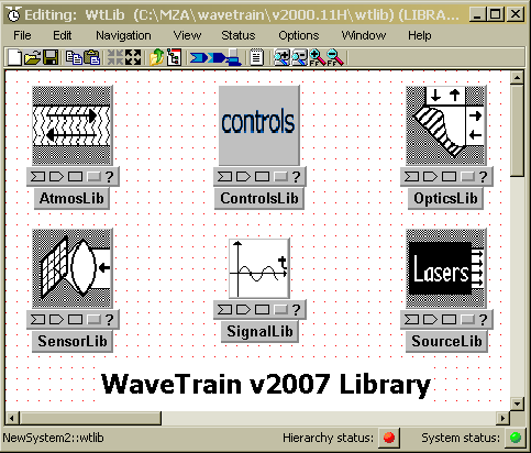
Figure: The WaveTrain component library, in WaveTrain Ver. 2007 and earlier
--------------------
All WaveTrain versions:
The above WaveTrain component libraries contain many different kinds of components (optical, electronic, and mathematical processing functions) that you need to model a wide variety of optical systems. The
WtLib library is the core WaveTrain library, while the other elements of the master library (equivalently, AllLibs) set contain components added to WaveTrain in more recent versions of WaveTrain. In the next section of this tutorial, you will descend into one or more of the WtLib sub-libraries, browse to find desired components, then copy and paste components into your new system.The six sub-libraries of the core
WtLib library are:Maximum allowed number of TVE System Editor windows
Above you opened two separate System Editor windows. In general, TVE allows you to open a maximum of three separate System Editor windows, which you can use for purposes of system inspection and editing.
Nomenclature note
In some places in the WaveTrain program suite and documentation, the "System Editor" may be called the "Block Diagram Editor (BDE)".
Copy components from one System Editor window to another
Now you will begin constructing your new WaveTrain system, by copying components from the WtLib library into your new system window. The order in which you copy the components make no difference, but it seems logical to start with a source. In the above System Editor window that contains the six sub-libraries, double-left-click the icon entitled SourceLib. This causes you to "descend" into the sub-library, so that you now see (in the same window) a variety of individual WaveTrain source modules (components) which have been collected for convenience into the sub-library. The window should look similar to the picture below, although the exact arrangement of the icons may differ. Note that in the picture below, the window size chosen for the illustration hides some of the individual components.
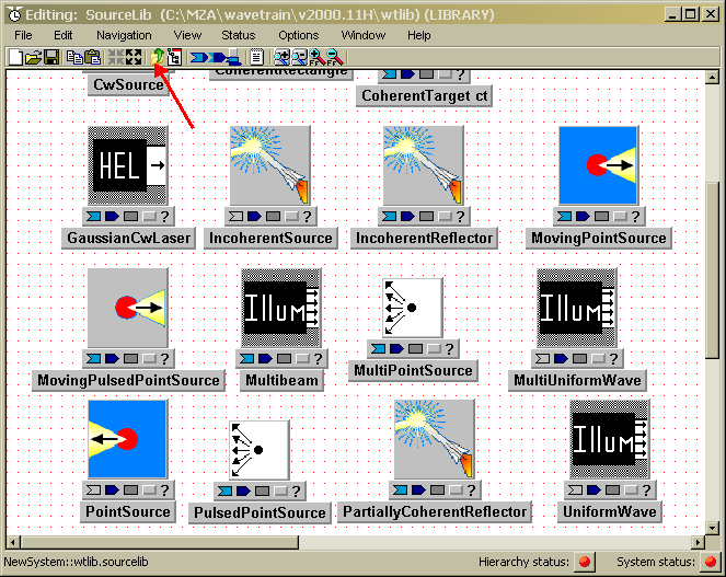
Figure: Contents of SourceLib (a sub-library of WtLib)
Note the toolbar button that is marked with the red arrow in the above figure. This button has Windows' standard "up-directory" icon: in the System Editor context, this signifies going up one level in a system hierarchy. If you left-click that button, you will return to the level that shows the six sub-libraries. Alternatively, you can go up one level by right-clicking on blank space in the editor window, then selecting "up one level" from the context menu. Double-left-click again on the SourceLib icon to descend again.
Now begin your system construction by copying the
PointSource component into
your blank new system window. The steps are:
(1) Find PointSource in the SourceLib
window.
Select PointSource
by moving the cursor over the icon and left-clicking. Notice this outlines
the icon in red.
(2) Use the window's menu bar to execute Edit - Copy PointSource.
(3) Move to the other System Editor window where you are building the new
system. In that window, go to the menu bar and execute Edit - Paste
PointSource.
(4) When first pasted, the icon may be jammed into the upper left
hand corner of the System Editor window. By left-clicking the icon and dragging it,
you can move it to any desired location within the window.
To select and paste additional components, simply repeat the copy-paste procedure for the additional components. In order to follow along with the illustrations and exercises in the remainder of this chapter, you should now copy and paste the remaining components in the following picture (you are building the same system as in the WtDemo system that was shown in the quick tour):
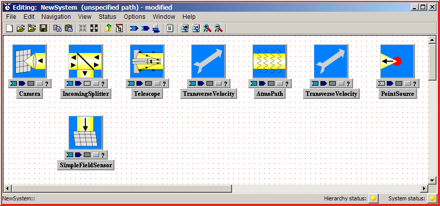
To find the components, you will want to access the
additional sub-libraries OpticsLib,
AtmosLib, and
SensorLib:
Component
Nomenclature: "components" in WaveTrain may also be called "subsystems", or "modules".
Appearance of the component icons
Do not be concerned if your component icons look somewhat different than the ones in the above figure: the icon pictures have occasionally changed during WaveTrain development cycles. However, the names of the systems in the title bars at the bottom of the icons should be identical! In fact, the icon pictures come in various flavors and color schemes, as well as various orientations. Later we explain how to modify the icons for aesthetic reasons, if desired.
The icon pictures should be interpreted loosely, and not taken too literally. For example, in the above picture the IncomingSplitter has the splitting interface oriented in the "wrong" direction for sending light to the SimpleFieldSensor. Such icon details have no functional effect whatsoever in the WaveTrain interface: it is only the connections that you will make between component blocks that determine where the light goes. Any component icon picture could be replaced by an arbitrary new picture with no effect whatsoever on system function.
Deleting a component
If you make a mistake, or are just experimenting, you can remove a component from your system by selecting it (left-click on the icon), and using the window menu sequence Edit - Delete. Alternatively, after selecting, right-click to get a context-sensitive menu that also presents a Delete option.
Alternate copy-paste procedures
As usual in graphical interfaces, there are alternate procedures available for copying and pasting. For example, once you have selected a component by left-clicking, then instead of using Edit - Copy from the menu bar, you can immediately right-click and obtain a context-sensitive menu that also offers the Copy command. Then, to paste the copied component into the new system window, you can right-click on blank space in the new window and obtain a context-sensitive menu that offers the Paste option.
It is also allowed to select more than one component at a time, using <Ctrl>-left-click to select the second, third, etc. components. The selected ones can all be copied at once and then pasted at once. When first pasted, they may all appear in the upper-left corner, stacked on top of each other. You can then drag them individually to their desired locations.
Saving systems, opening existing systems
Saving
At this stage, save your new
system before proceeding to the next stage of system construction. A system
can be saved at any stage; no particular level of completeness needs to be
achieved before saving . To save the new system, the steps are:
(1) In the System Editor window menu bar, left-click File - Save As.
(2) Navigate to any directory where you want to store your system.
(It would be preferable to not use any tempus or WaveTrain
subdirectories).
(3) Specify a system (file) name of your choice, and press Save.
The file extension .tsd (tsd = "tempus system definition") will be
automatically appended to the name you specify.
In older versions of WaveTrain, File - Save As may first place you in a WaveTrain library directory: you do not want to save your system there. Wherever you choose to save it, it is usually good practice to store each new WaveTrain system in its own directory, because the process of building the system, the runset and then executing the runset will generate numerous files associated with one system.
Once the new system has been saved for the first time, subsequent changes can be saved by using just File - Save.
Opening an existing system
Suppose that you wish to work with a system that has been
previously saved, but is currently not open in a System Editor window. To
do this, the steps are:
(1) Open a new System Editor window from the TVE toolbar.
(2) In the editor window menu bar, left-click File - Open - Browse.
(3) In the resulting directory window, navigate to the directory where the
system of interest is stored.
(4) Select the .tsd file that bears the system name you want, and
press Open (or just double-left-click the .tsd file name).
(*) As an alternative to File - Open - Browse, the menu sequence File - Recent systems is also useful: this presents you a quick list of systems that you've recently opened.
The present TVE environment allows a maximum of three separate System Editor windows to be open at one time.
Next steps in building your system
After you have copied or added the desired subsystems into your new or working system window, you will need to set their parameters, and connect them together. In general, these steps can be done in either order.
Component parameters, inputs and outputs
After you copy or add components (subsystems), you will need to assign values to their "parameters", and possibly to some of their "inputs". These two terms are used in a specialized sense in WaveTrain: they are both inputs in a generic sense, but the distinction is that "parameters" are fixed in time, whereas "inputs" may or may not change with time.
A typical component "parameter" might be an aperture diameter, a source power, or a mesh spacing.
A typical component "input" might be a "wavetrain" (WaveTrain's data structure that carries the optical field information). The data in a wavetrain incident on a component usually changes as the simulation time advances. On the other hand, timing parameters that define sensor exposures are also "inputs", even though most of these do not change with time.
A typical component "output" might be a wavetrain, or a time-integrated sensor exposure map.
A component may have any number of parameters, inputs and outputs. A parameter must be assigned a value. An input usually receives its value by being connected to the output of another block, but sometimes an input is assigned a value explicitly. Outputs are usually connected to the inputs of other components; in some cases, outputs are not graphically connected to anything, but may just be recorded. These options will become clearer as you continue with the construction of the tutorial system.
In the subsequent sections of this introductory tutorial, you will see many examples of parameters, inputs, and outputs. We will refer to them without quotes from now on; it should be clear from the context whether "input" is meant in the specialized WaveTrain or the generic sense.
Display/hide graphical elements
Before actually setting any parameters or connecting inputs and outputs, you must become familiar with certain mechanics of the graphical user interface (GUI) related to displaying and hiding of the component graphical elements. Notice that, in the copy-paste operations you performed above, the component (subsystem) icons consisted of a picture, a miniature toolbar beneath the picture, and a component name bar below that.
Displaying/hiding the components parameters, inputs and outputs
Due to the finite display space available, it is
frequently useful (or necessary) to hide various graphical elements. Of
course to initially set the parameters and to connect the inputs and outputs,
these items must be displayed.
 To
display or hide, you will use one of the toolbars buttons in the System Editor
window, and also the miniature toolbars located underneath the component icons.
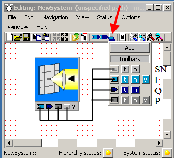
The master control for displaying and hiding is the toolbar button indicated by
the red arrow in the picture at right. In the new system window in which
you have been assembling your system, left-click the indicated button.
That pulls down the palette which you see in the picture at right. This
palette contains six rows of buttons: for now we are just interested in the last
four rows, each of which consists of three or four small buttons. The
first of these rows is labeled "SN" in the picture, and controls display of
System Names. The second row, labeled "I" in the picture, controls display
of Inputs. The third row, labeled "O", controls display of Outputs.
The fourth row, labeled "P", controls display of Parameters.
To
display or hide, you will use one of the toolbars buttons in the System Editor
window, and also the miniature toolbars located underneath the component icons.
The master control for displaying and hiding is the toolbar button indicated by
the red arrow in the picture at right. In the new system window in which
you have been assembling your system, left-click the indicated button.
That pulls down the palette which you see in the picture at right. This
palette contains six rows of buttons: for now we are just interested in the last
four rows, each of which consists of three or four small buttons. The
first of these rows is labeled "SN" in the picture, and controls display of
System Names. The second row, labeled "I" in the picture, controls display
of Inputs. The third row, labeled "O", controls display of Outputs.
The fourth row, labeled "P", controls display of Parameters.
Global display/hide: As an initial exercise, after pulling down the palette, left-click on the leftmost "I" button: in your new system window, you should now see that the inputs of all your components are now displayed. The display may be messy because the icons are too close to each other for present purposes. Grab one or two of the icons and move them to see everything for those icons. The palette buttons are all "toggles", so click the same button again to hide the inputs. The leftmost button in the "O" row serves the same function for component outputs, and the leftmost "P" button serves that function for the component parameters. Any combination of I,O, and P may be displayed. Finally, note that the leftmost "SN" button allows you to turn off/on the display of component (system) names; these take less room, so usually there is not much point in hiding the names.
Individual component display/hide: Instead of
applying the display/hide toggles to all components at once, it is often
very helpful to apply the toggles to one component at a time. To do this,
simply select (left-click) the icon of interest, and then press the
above-discussed palette buttons.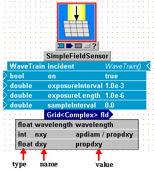
Displaying/hiding type, name, value elements: Next, consider the palette buttons labeled "t" (= type), "n" (= name), "v" (= value). Each of the SN, I, O, P rows in the previous figure has such buttons. As an exercise, select the SimpleFieldSensor icon in your new system, and use the palette buttons in the leftmost column to display inputs, outputs, and parameters. When all elements t, n, and v are displayed, your component should look like the illustration at right. Note that inputs (light blue fields) and parameters (light grey fields) have three columns: type, name, and value, as indicated by the red arrows. Outputs have only two columns: t and n. You can use the subsidiary palette buttons labeled t, n, and v to display/hide any combination of individual elements of the I, O, P fields. Until you become more familiar with the significance of the elements, it is probably best to display all elements or none.
Miniature toolbar under component icon: From inspection of the above picture, you will see a miniature toolbar directly below the component icon, above the component name. The mini-toolbar has symbols that look exactly like the buttons in the left column of the palette. Once you have used the palette to set the display/hide properties of the t, n, v elements to your liking, then you can more quickly display/hide the SN, I, O, P rows by just left-clicking the mini-toolbar buttons. Note that clicking the mini-toolbar buttons preserves the t, n, v settings that you have chosen with the palette.
The component name fields: We have not yet
said much above about the SN row of the palette, and the display fields that it
controls. The system (component) name fields have a different function
than the I, O, P fields, although the display/hide features are controlled in
exactly the same way using the palette and the mini-toolbar. The example
at right shows one of the
TransverseVelocity components from the new system that
you have assembled. 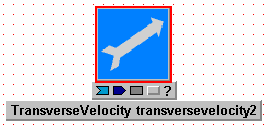 We have used the palette buttons to display both t and n for the SN row, and we
have hidden the I, O, P rows. The t (type) field in the SN bar corresponds
to what is technically called the "C++ class name" in the WaveTrain code.
The text in this field, "TransverseVelocity", is
not user-editable. The n (name)
field in the SN bar is also assigned by default when you insert the component
into your system. However, the text in the n field is arbitrarily
adjustable by the user. There is usually no need to make any
adjustment to the default assignment, but this name can be changed to conform to
user preference. A significant point is illustrated by the example at
right. Note that the System Editor assigned the default name
"transversevelocity2".
That is because we inserted two
TransverseVelocity
components into our new system, and this was the second "instance" of the
TransverseVelocity
type that we inserted.
You are allowed to change the name and suffix number to anything that seems
meaningful or convenient to you, by clicking on the name and editing. The
numbering need not be consecutive, or you can just use different names and no
numerical suffix: the only requirement is that multiple instances of a
"class" must have distinct names.
We have used the palette buttons to display both t and n for the SN row, and we
have hidden the I, O, P rows. The t (type) field in the SN bar corresponds
to what is technically called the "C++ class name" in the WaveTrain code.
The text in this field, "TransverseVelocity", is
not user-editable. The n (name)
field in the SN bar is also assigned by default when you insert the component
into your system. However, the text in the n field is arbitrarily
adjustable by the user. There is usually no need to make any
adjustment to the default assignment, but this name can be changed to conform to
user preference. A significant point is illustrated by the example at
right. Note that the System Editor assigned the default name
"transversevelocity2".
That is because we inserted two
TransverseVelocity
components into our new system, and this was the second "instance" of the
TransverseVelocity
type that we inserted.
You are allowed to change the name and suffix number to anything that seems
meaningful or convenient to you, by clicking on the name and editing. The
numbering need not be consecutive, or you can just use different names and no
numerical suffix: the only requirement is that multiple instances of a
"class" must have distinct names.
Now that you have mastered the displaying and hiding of
display elements, you are ready to set the parameters.
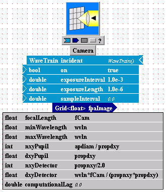
In your new system, select the SimpleFieldSensor component, and display all the I, O, and P
elements to follow along. After you've copied SimpleFieldSensor from WtLib,
and you've displayed all the elements, it
should look like the illustration at right.
Note: Depending on the age of your WaveTrain version, there may be
some differences in the contents of the rightmost "value" column.
We now want to enter desired values in the value fields (rightmost column) of the parameter block (light grey) and the input block (light blue). In WaveTrain, we use the term "setting expression" to denote the expression entered in a value field. Note that in this example all the value fields are already filled in with some default setting expressions. This will not be the case with all components: sometimes the value fields are initially blank. In either case, these initial settings are usually not what you want in your new system.
Note that some setting expressions in the picture are simple numbers ("1.0e-3"), some are symbols ("wavelength", "propdxy"), some are boolean expressions ("true"), and some are algebraic expressions ("apdiam / propdxy"). After you finish the introductory tutorial, you can obtain full details on the expressions and functions that are allowed in setting expressions by referring to the detail chapter on Data Entry.
The simplest method of assigning a setting expression is
to enter a number. If you enter a number and press <return>, you are
completely done with that parameter. However, this is often
undesirable for two possible reasons:
(a) You may want to link the value to that of another parameter value.
(b) You may want to vary the value later at the level of the WaveTrain
Runset Editor (to be discussed later in this chapter).
To handle issues (a) or (b), you must assign a symbolic name or algebraic
expression as the setting expression.
To change or initially assign a setting expression, left-click in the value field of interest and begin typing. A few rudimentary text-editing features are available, e.g. text selection and copy-paste via <ctrl>-C and <ctrl>-V. Press <Enter> to complete the edit. You will now practice entry of setting expressions by changing or accepting all the value fields of SimpleFieldSensor:
Enter setting expressions for SimpleFieldSensor:
(1) Parameter name "wavelength":
(*) Currently, the value of this parameter is
also "wavelength". For practice, enter the new setting expression "wvln".
Note: you are allowed to use the same symbol for a parameter setting as
the parameter name, or a different one: the default here was the same, but
you just changed the value to "wvln".
(*) When you pressed <Enter>, the System Editor
popped up another window, entitled "Expression Contains Undefined Identifiers",
as shown below. Press the button "Add as Parameter" to register the symbol
"wvln" that appears in the "name" column:
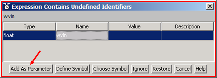
CAUTION: symbols inside the WaveTrain program are case-sensitive. E.g., "Wvln" is different than "wvln", etc.
(2) Parameter name "nxy":
nxy and dxy define the space mesh on which SimpleFieldSensor will report its
results. Let's just accept the default expression "apdiam / propdxy" that
is already present:
(*) Left-click in the value field, and simply
press <Enter>
(*) Note that the System Editor again pops up the
"Undefined Identifiers" window: press "Add as Parameter" twice to register
the symbols "apdiam" and "propdxy".
The two parameters "apdiam" and "propdxy" will refer to key properties of two other components, namely Telescope and AtmoPath, respectively.
(3) Parameter name "dxy":
Again, let's just accept the default expression:
(*) Left-click in the value field, and simply
press <Enter>
(*) This time, the System Editor does not
produce the
"Undefined Identifiers" window: that is because the symbol "propdxy"
has already been registered in the previous step, when you defined the setting
expression for parameter name "nxy".
In the
SimpleFieldSensor
module, the last four inputs (in addition to the parameters) also require
setting expressions. On the other hand, the input of type "WaveTrain" will
receive its input by being connected to the output of another block, so we enter
nothing in the value field of that first input bar:
(4) Input name "on":
(*) Left-click in the value field, and simply
press <Enter>
(*) The boolean symbol "true", which you've just
accepted, is already a defined in the WaveTrain code, so the "Undefined
Identifiers" window did not pop up.
The "true" setting means that the sensor's first exposure window will start at simulation time t=0.
(5, 6) Input names "exposureInterval",
"exposureLength":
These names mean exactly what they say: they define, respectively, the interval
between start of successive exposure windows, and the length of each exposure
window. All the basic WaveTrain sensors are time-integrating sensors,
although later you may encounter sensors that directly report power or
irradiance.
(*) Accept the default numerical values for these
two timing inputs.
Numerical values in the WaveTrain program are in MKS
units, unless explicitly specified otherwise: all time quantities are in
seconds.
(7) Input name "sampleInterval":
This name may be a little confusing. It allows you to perform multiple
WaveTrain propagations during each exposureLength window.
(*) Leave it set at 0.0 for this tutorial:
that means that the optical field at the sensor will be computed once during
each exposureLength.
After completing the introductory tutorial, you can consult the detail section Sensor Timing and Triggering for further information about timing options.
Parameters sub-window:
Before proceeding with the setting expressions for other components, you should now become aware of a sub-window of the System Editor. Using the System Editor View menu, execute the menu commands View - Parameters. This makes visible a sub-window within the System Editor, which we call the Parameters Panel, as shown in the following picture:
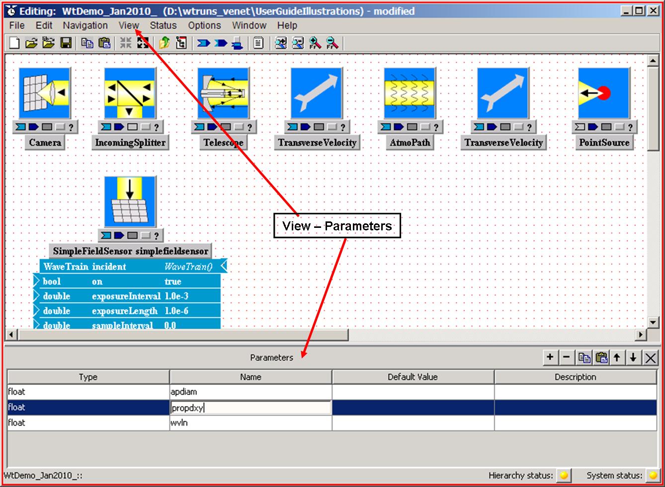
The Parameters Panel contains a listing of all the symbols that you have
defined so far: "wvln", "apdiam", and "propdxy" all appear. If
undesired symbols still appear in the list (e.g., from some experimentation you
might have done), you can (and should) delete those by left-clicking in their
row, and pressing the
![]() button at the top right of the Parameters Panel.
button at the top right of the Parameters Panel.
For now, let's ignore the "Default value" and "Description" columns in the Parameters Panel. You can toggle the Parameters Panel display on and off, as convenient, using View - Parameters.
Help pages for individual WaveTrain components
In this tutorial, we guide you by giving you valid setting expressions to
enter for all parameters and inputs. Naturally, when you eventually do
this on your own, you will need reminders of the meaning of, and valid possible
settings for, the many component parameter and input names. This information
can be obtained for each component by left-clicking the question-mark button,
![]() , at
the bottom right of any component icon.
, at
the bottom right of any component icon.
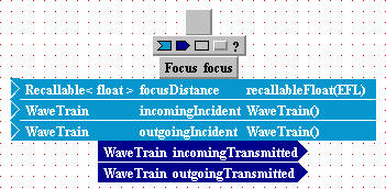
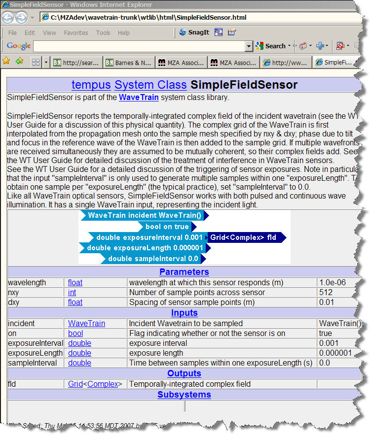
Try this, for example, with the SimpleFieldSensor component whose settings you entered above. You will see that a HTML help page opens in your web browser: this page contains a summary description of the component's function, and short physical definitions of each parameter, input and output. Sometimes these descriptions may be terse, and you may still have to consult sections of the User Guide for interpretation. Nevertheless, the component help page is the place to start.
The picture below shows the help page that you should see for SimpleFieldSensor: .
Enter setting expressions for remaining components:
At this point, you have completed the setting expressions for the SimpleFieldSensor module, and you should now enter the setting expressions for the remaining components as follows.
Enter setting expressions for PointSource:
Initially, PointSource copied from
Wtlib has the default values shown below.
(*) Since we decided above to represent the
propagation wavelength by the symbol "wvln", you should change the symbol
"wavelength" in the value field to "wvln".
(*) Accept the default numerical values of the
other parameters as they are.
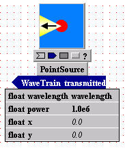
(Note that the PointSource parameter named "power" is poorly named: this parameter is actually the Watts/steradian produced by PointSource).
Enter setting expressions for TransverseVelocity (first instance named transversevelocity, and second instance named transversevelocity2):
You will assign the parameter values to represent a uniform atmospheric
wind speed, transverse to the propagation path, with stationary source and
receiver. (Picture the three velocities with respect to an earth frame,
which is considered inertial).
(*) Change the default settings to match those
in the pictures below:
![]()
![]()
Notice that we have entered "vWindX" in one motion module and "- vWindX" in the other. To understand the physical meaning of these settings (after completing the present tutorial), you can consult the User Guide detail sections for further information about the specification of transverse displacement and transverse motion in WaveTrain.
Enter setting expressions for AtmoPath:
This is a complicated component, with many parameters. AtmoPath contains specifications for both the Fourier propagation mesh and the turbulence phase screen parameters. For present tutorial purposes, we will enter settings here without explaining all the details. The details can be learned later by consulting various sections of the Modeling Details section of the User Guide.
Parameter name "atmSpec":
This parameter contains most of the settings that define the atmospheric
turbulence along the propagation path. The setting expression in this
value field is something new compared with the components you worked with above:
it is a special function, "AcsAtmSpec(...)",
that is part of the WaveTrain code. You will now set the arguments of this
function:
(*) Left-click in the value field, and change
"wavelength" to "wvln", to accord with your previous symbol definitions.
(*) Press <Enter>, and you will once again see
the "Undefined Identifiers" window. Left-click the "Add As Parameter"
button five times, to register the remaining default symbols that appear in the
argument list, namely "nscreen, clear1Factor, hPlatform, hTarget, range".
We will briefly discuss the physical significance of these symbols later in the
tutorial, when we finally assign them numerical values.
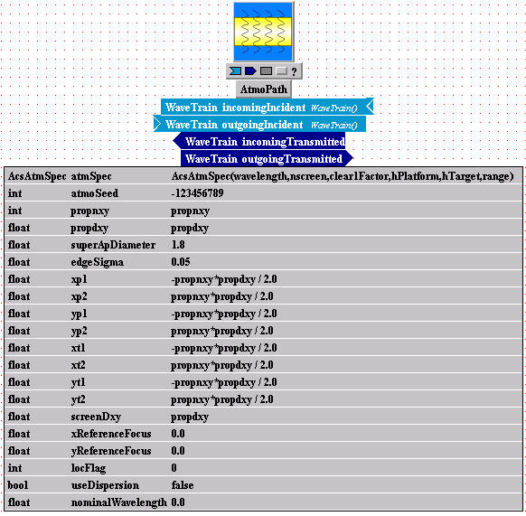
Parameter name "propnxy":
Parameter names "propnxy" and "propdxy" define the size and spacing of the mesh
that WaveTrain will use for its Fourier propagations. Obviously, these are
critical specifications.
(*) Left-click in the value field, press
"<Enter>, and "Add As Parameter" to accept the default symbol "propnxy".
(You already defined the symbol "propdxy" in a previous component").
Parameter names "xp1" through "yt2", and "screenDxy":
These parameters define the dimensions and mesh spacing of the turbulence phase
screens. The symbols in the respective setting expressions have all been
registered previously, so you need do nothing here.
Remaining parameter names:
The setting expressions are either numerical values, or symbols previously
defined. You will accept all these for now, so no further action is
required to complete the AtmoPath
settings.
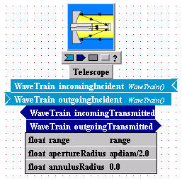
Enter setting expressions for Telescope:
This component performs two functions: (a) it applies a binary aperture (in general, annular), and (b) it undoes the wavefront curvature acquired due to propagation from a point source to the telescope. Function (b) works together with the Camera module that follows.
Parameter name "range":
Here you simply enter the distance to an OBJECT plane whose image you
want to generate in the focal plane of a subsequent Camera module:
(*) The desired setting expression in the value
field, "range", is already present by default, and you have previously
registered this symbol. No further action is required.
Parameter names "apertureRadius" and "annulusRadius":
(*) These already have the desired setting
expressions entered by default, and the symbol "apdiam" has been registered
previously. No further action is required.
Note the mixed nomenclature: "apertureRadius" signifies the outer radius
of the annular aperture, while "annulusRadius" signifies the inner
radius, all in MKS units (i.e., meters).
No setting expressions required for IncomingSplitter
This component makes a copy of the incident wavefront and retransmits it into two separate optical paths. Note that the wavefront is duplicated: it is NOT split in energy.
Enter setting expressions for Camera:
Patience,
you're almost done!(*) Edit the setting expressions in Camera's parameter value fields to match the picture below.
(*) One CAUTION: the parameters named "nxyPupil"
and "dxyPupil" unfortunately have quite misleading names. Unless you
explicitly use an esoteric feature of WaveTrain ("wavesharing"), these parameter
values are NOT used in the calculation. The aperture which controls the
diffractive spreading in
Camera's image is the
Telescope aperture that you specified above.
(*) The setting expression you entered for the
parameter named "dxyDetector" exploits the full resolution available from
Execute the menu commands File - Save
Of course, you can do this at any time during the above work, but make sure you do so before proceeding to the next stage of construction.
You have now completed the entry of setting expressions for all your component parameters. At this point, you should verify that the settings are complete, and furthermore, syntactically consistent. The mechanism provided by WaveTrain to perform this check is the pair of status bulbs at the bottom right of the System Editor window
Status bulbs
At the bottom right of the System Editor window, you will
see the two status indicators
![]() and
and
![]() . The two colored bulbs can be either red, yellow or green, indicating various
levels of missing or inconsistent information in the parameter and input setting
expressions.
The "System status" bulb refers to the system level currently displayed in the Editor
window: this is the one of present interest.
. The two colored bulbs can be either red, yellow or green, indicating various
levels of missing or inconsistent information in the parameter and input setting
expressions.
The "System status" bulb refers to the system level currently displayed in the Editor
window: this is the one of present interest.
If the status bulbs are not green, it means that one or more problems have been detected by the TVE. In the system you are constructing, left-click on the "System status" bulb, which should be green at this point. A message box will pop up, telling you that no problems are detected at this time.
Now that you have completed the setting expressions for all the components of
your tutorial system, the next step is to connect the components together.
This step is very simple: to connect the output of one component to the input
of another component, you must:
(a) Make sure you display the inputs
and outputs of the components you want to connect.
(b) Place the cursor on the arrowhead of a dark-blue output bar: the
arrowhead should turn red when you are over the sensitive region.
(c) Left-click and drag to the connection triangle at the end of the
desired light-blue input bar,
and release: a connection line will appear.
Carry out steps (a)-(c) to make the connections shown in the following figure:
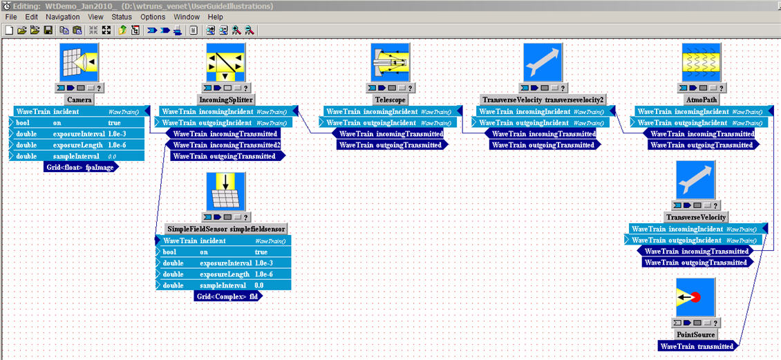
In producing the above layout, we've used several GUI features to improve
the visual presentation:
(a) You can spread out the component icons to give more room, either by
dragging the individual icons, or by pressing the "unpack"( ![]() ) and "pack" (
) and "pack" (![]() ) buttons in the
System Editor toolbar.
) buttons in the
System Editor toolbar.
(b) You can introduce bends in a connecting line, by left-clicking on a
line and dragging (right-click and "delete vertex" to undo).
(c) The connection triangles or arrowheads of inputs and outputs may be
flipped from one side to the other of the colored bars. To
do so, place the cursor on a colored bar and double-left-click.
Alternatively, place the cursor on a bar and right-click to get a
context-sensitive menu, then "Flip".
(d) The horizontal and vertical layout of components is completely
immaterial to their functionality: only the connections control which way
light is going. (A later Guide section explains
details of coordinate and
direction conventions).
After all components are connected and setting expressions defined, you may want to hide all inputs,outputs and parmaeters, leaving just the connecting lines showing. In that case, your completed system could be compacted as follows:
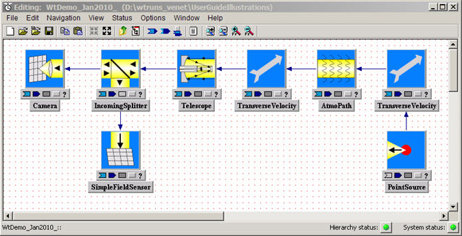
Note that all your connecting lines are single-headed arrows: that is because light is only going in one direction in this tutorial system. In many systems, you will have light going in both directions ("incoming" and "outgoing", in WaveTrain nomenclature).
At this stage, you can always redisplay the inputs, outputs, or parameters of individual components as needed.
Execute the menu commands File - Save
Of course you can do this at any time during the above work, but make sure you do so before proceeding to the next stage of construction.
Create a new run set for the WaveTrain system
Now that you have completed assembly of your WaveTrain system in the System Editor, you must create a "run set" for it. After the run set is created, you will be able to compile and run the simulation with two button clicks.
To create a run set for your system model, go to the
System Editor file menu and
(*) execute File - New - Runset;
(*) in the input box that pops up, enter a name of your
choice (say, "A") for your new run set;
(*) press "OK".
In general, the run set name can be constructed from any combination of letters, numerals, and the
underscore character. The data eventually
generated by running your simulation will be stored in an output file
named according to the pattern "SystemNameRunRunSetNameK.trf",
where
SystemName
= name of the WaveTrain system (user-specified)
Run = prefix inserted by the WaveTrain code
RunSetName
= name of the run set (user-specified)
K = a
sequential numerical index assigned by the WaveTrain code
.trf = extension designating a specially-formatted data file (pronounced "turf" by
WaveTrain initiates).
When you pressed OK to create the new run set, you obtained a new editor window that has the appearance shown below. This is called the Run Set Editor window. The acronym "TRE" in the window title bar stands for the full name "tempus Run Set Editor". In the title bar of the window, you will see the name you assigned to the run set, followed by (in parentheses) the directory path and name of the system with which it is associated.
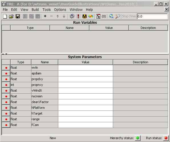
Notice there are two panels in the Run Set Editor:
(a) the Run Variables panel, currently blank;
(b) the System Parameters panel: notice that the parameter names
that appear here are precisely those symbols that you defined when you entered
them previously in the component setting expressions of the system editor
window. You can verify that the name list here exactly matches the
comprehensive name list that appears when you View - Parameters in the
System Editor window.
You must now do the following four things in the Run Set Editor
before you can finally run your simulation:
(a) Assign numerical values (or file sources) to the System Parameters
(b) Possibly define some Run Variables
(c) Enter a simulation Stop Time
(d) Specify one or more variables for recording.
Assign numerical values to System Parameters and Run Variables:
(*) Left-click and type in the "Value" fields of the
System Parameters panel, and assign the values shown in the modified picture
below.
(*) Press <Enter> to accept a value setting before moving to another entry
field
Physical units: inputs, outputs and parameters in WaveTrain are in MKS units. One caution on units: phase or OPD inputs/outputs can be a little tricky, in that different components may assume meters or radians, which will be specified by the help page for the individual components.
(*) Parameter name "nscreen" needs a special
adjustment:
This adjustment is required due to a deficiency in the WaveTrain interface.
We include this bit of ugliness in the tutorial because it will appear in
practically every atmospheric propagation model, and you must get used to it.
Notice that in the original Run Set window above, and in the
System Editor window upon which the run set is based, the editor assigned the
data type of "float" to the symbol "nscreen". But this is incorrect,
because "nscreen" represents the integer number of phase screens in the
atmospheric turbulence model. If you go back to the
AtmoPath component
in the System Editor, you can see that you first entered "nscreen" as an
argument in a function, AcsAtmSpec(..., nscreen, ...). In that kind of
setting expression, and only that kind, the editor is unable to determine the
correct data type for the function arguments, and just labels them all as
"float" type. You must manually correct by doing the following:
(i) In the Parameters Panel of the System Editor,
left-click in the "Type" field of the "nscreen" parameter, and replace "float"
by "int". Press <Enter>.
(ii) Still in the System Editor, execute the menu commands
File - Save.
(iii) In the pop-up box that now appears, click "Yes" to update the
open runset. You will see that the "Type" of "nscreens" in the Run Set
window has now updated to "int".
After the above manipulations, your runset should look like the following figure:
Execute the menu commands File - Save:
In the Run Set Editor window, execute the menu commands File - Save. Proceed with saving despite the resulting "incomplete" warning.
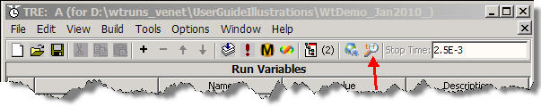
Enter a simulation Stop Time:
In the upper right of the Run Set Editor, find the box called "Stop Time". All WaveTrain simulations start at t=0, and run until the designated Stop Time (in seconds). Whether and when any calculations are done during t=[0.0, Stop Time] depends solely on the sensor timing parameters that you defined in the sensor components of you system. In the above system, you've included two sensors,
SimpleFieldSensor and Camera, and you assigned them identical timing parameters. Specifically, you set the sensors to take exposures starting at intervals of 1 msec, with an exposure length being 1 msec.(*) Enter the value 2.5E-3 (seconds) in
the Stop Time box.
This will produce three exposures, because the first one starts at t=0.
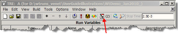
Specify variables for recording:
When you execute the simulation, WaveTrain records no results by default. You must specify precisely which outputs you want to record.
(*) In the Run Set Editor, press the Recorded Outputs button in the toolbar, where indicated by the red arrow in the following figure:
A new window will pop up, entitled "Output Recording" as shown below, which contains a listing of all the component outputs that are available for recording.
(*) Click on both check boxes: this will cause
recording of the camera and field sensor output maps (one map for each exposure
window in each sensor)
(*) Note that below the check boxes, the radio button "When changed" is
selected". This is the usual choice; leave all other boxes
unchecked.
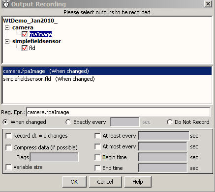
(*) Press "OK" to accept your selections and to close this window.
Notice that the "Output Recording" button in the Run Set Editor toolbar now
has the anotation "(2)", indicating that two output variables have been selected
for recording.
Notice also that the status bulbs at the bottom of the Run Set Editor are now
both green, implying that all required settings have been filled in, insofar as
the Editor can determine.
Execute the menu commands File - Save:
In the Run Set Editor window, execute the menu commands File - Save.
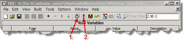
(*) Press the "Compile and link" button in the Run Set Editor (see red arrow #1 in the screenshot below).
A Windows console window will appear, and
some messages will be generated that are useful for debugging in case there are
still setup errors in your system or runset. (The messages will be useful
once you acquire some more experience with WaveTrain). The tutorial system
you've constructed should have no errors at this point, so the console messages
should conclude with:
" Created executable "SysNameRunRunName.exe"
with optimization (Release version).
Make completed successfully
Press any key to continue . . ."
Press any key to close the console window.
(*) Press the "Execute simulation" button in the Run Set Editor (see red arrow #2 in the screenshot above). As a result, two things will happen:
(i) Another Windows console window
will appear,
containing messages that show the progress of the simulation run. These
messages are not particularly informative to WaveTrain users. Your
tutorial system system should complete execution in a few seconds at most:
you should then see the message "execution complete"
in the console window.
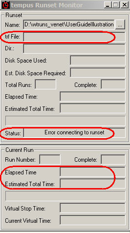
(ii) A separate small diagnostic window, entitled "tempus Runset Monitor",
will appear. This window is shown at right.
Your tutorial system will most likely finish too fast for the Runset Monitor to
latch on to the process and begin acting. As a result
the Monitor will report that there was an "Error connecting to runset",
as shown in the picture at right in the second red-circled field. Just
ignore this, and close the Monitor window.
If you are executing a run set that
requires more time, the Runset Monitor may provide some useful diagnostics.
First, the Monitor will report the name of the *.trf file that WaveTrain
created (in particular, the auto-generated numerical index): see the first
red-circled field at right. Lower down in the Monitor, there is a panel
entitled "Current Run", which tells you the run
number currently in progress. Just below that, there are panels that
report the elapsed wall-clock time, and the estimated time remaining to complete
execution of the run set. The latter estimate is typically fairly
accurate, but is not foolproof, because its accuracy depends on the structure of
the looping calculations in the runset.
You will now use WaveTrain's TrfView viewer to inspect the recorded simulation results.
Start the TrfView viewer:
(*) Press the "TrfView" button in the Run Set Editor toolbar, where indicated by the red arrow in the screenshot below:
The preceding button press opens the TrfView viewer, and also locates and opens your most recently generated *.trf file. (This *.trf file contains your recorded simulation results). The main window of TrfView then appears, which will look as follows:
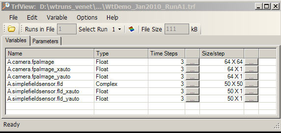
The "Name" column contains the names of all
the variables that you checked for recording in the "Ouput Recording" menu of
the Run Set Editor: note the presence of
"A.camera.fpaImage"
"A.simplefieldsensor.fld".
The "A" prefix is the run set name, which may differ depending on what you named
your run set.
(If you want to inspect data from a different *.trf file, you can go to the TrfView file menu and execute File - Open ... to navigate to and select a different *.trf file name. You can only inspect one *.trf file at a time).
Plot recorded data in TrfView:
(*) Right-click on variable name "A.simplefieldsensor.fld"
to get a context menu
(*) Click "Plot variable"
You should now see the following plot window:
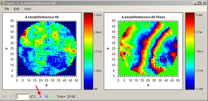
This shows the amplitude (left panel) and
phase (right panel) of the complex field recorded by the SimpleFieldSensor
component. Key feature of the plot window are:
(i) The x and y axis scales are in sensor pixel units.
(ii) The phase of the complex field is in radians.
(iii) The amplitude units are a more complicated issue (read the detail sections
on units and sensors
for full discussion).
(iv) The button marked by the red arrow in the picture controls which
sensor exposure (which time step) you are plotting. Currently the window
is showing exposure "1 of 3". Press the button (and its companion buttons)
to cycle among the exposures. Note how the plot appears to (approximately)
translate as you move in time: this reflects the fact that the wind speed
setting in your system causes the phase screens to translate.
(v) The small panel labeled "Time", to the right of the exposure buttons,
tells you the exact simulation time at which the sensor exposure data became
available. In the system that you created, the end of the exposure windows
occurred at t = (0+1.0msec,
1.0msec+1.0msec,
2.0msec+1.0msec), i.e., at
t = (1.0msec, 1.001msec,
2.001msec). This is precisely what the "Time" panel reports as you cycle
among the exposures.
(*) Click and plot the variable "A.camera.fpaImage"
for further practice.
This variable is the temporally-integrated
irradiance (units of J/m2), in the camera focal plane.
(*) Magnify (zoom in on) a section of the plot, by left-clicking and
dragging to outline the section that you want to magnify. To undo the
zoom, right-click in the plot and select "Unzoom".
(*) New as of WaveTrain 2010A: In addition to the variables "A.camera.fpaImage" and "A.simplefieldsensor.fld", the TrfView main window pictured above also listed companion variables "..._xauto" and "..._yauto". These variables automatically record mesh geometry information.
The *.trf file itself:
When using TrfView, the viewer manages all
the opening, closing and reading of the *.trf data files. As you
become a more experienced WaveTrain user, you will want to deal with these files
in other ways than TrfView alone. For now, just verify that the trf file
appears in the same directory where you saved the WaveTrain system.
Remember that the trf file was named according to the pattern
"SystemNameRunRunSetNameK.trf"
In the present case, the suffix K=1 was assigned by WaveTrain, because it was
the first *.trf file having the specified system name and runset name in
the directory.
Suppose you now went on to change some entry values in the System and/or Run Set Editors, resaved your run set under the same name, and executed the simulation again. Then WaveTrain would create a new *.trf file with the K index incremented by 1. Thus, there is never any danger of WaveTrain overwriting previous *.trf files.
Congratulations!
You have completed the creation and running of your first complete WaveTrain simulation!
At this point, there are several additional
topics in WaveTrain system construction which you should work through as an
extension to the introductory tutorial. The following procedures are
typically needed, or at least desirable, even in simple WaveTrain systems:
(a) Inserting a loop variable in the Run Set editor
(b) Elevating parameters
(c) Changing the list order of System Parameters
(d) A few clean-up procedures
(e) Basic documentation using the "Description" fields in the Editors
Multiple run sets for a given system
You can create an arbitrary number of run sets for the same WaveTrain system. (Recall that to create a runset, you execute File - New - Runset in the System Editor where you have the WaveTrain system open). The multiple run sets are distinguished by the user-specified names that you assign. Multiple run sets give you some organizational freedom to set up different sets of inputs while minimizing the amount of text editing required in the Run Set Editor. To assist in populating the setting expressions in closely-related but lengthy run sets, there is a File - Import option in the Run Set Editor.
Previously in the tutorial, you have created and executed a WaveTrain system based on a single set of parameter values. (Although, remember that you had wind motion in your system, so there was already changing behavior in time due to phase screen motion). Now, you will insert a "loop variable", which will allow you to repeat the time sequence of sensor exposures for several values of the designated loop variable.
A loop variable can control any parameter in the setting expressions of your system components. For example, you could repeat the whole time sequence of sensor exposures for several values of an aperture diameter, leaving all other parameters fixed. Wavetrain permits multiple (nested) loop variables, but for this tutorial we will illustrate the procedure with a single loop variable.
A frequent desire in WaveTrain analyses is to repeat a simulation for many (or at least several) statistical realizations of atmospheric turbulence. You will now add a loop variable to your previously constructed tutorial system to accomplish this.
(*) If necessary, start Wavetrain and
open your previously-saved tutorial system.
(*) In the System Editor window, display the parameters of component
AtmoPath.
(*) In the row for parameter name "atmoSeed", replace the current setting
expression "-1234567" by the symbol "atmoSeed", as shown in the picture below.
Remember to press the "Add As Parameter" button in the "Undefined Identifiers"
pop-up window.
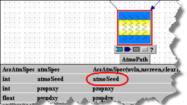
(*) File - Save your modified system.
(*) If necessary, open a Run Set Editor
window from the TVE toolbar,
and use File - Open to select and open the run set that you previously
created. The editor presents you with a restricted browse window that only
shows run set names. When preparing the tutorial illustrations, we called
our run set "A", as indicated in the picture below. Select and open the
name that you assigned.
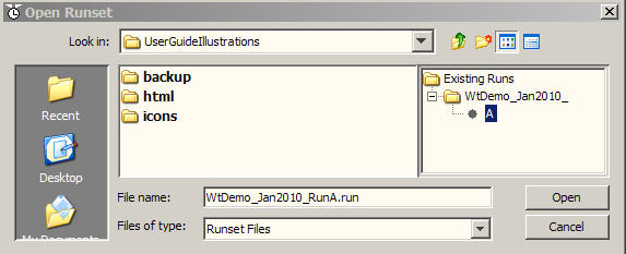
(*) Now that your run set is again
open, in the status bar at the bottom of the window you will see the warning
"Obsolete": that occurs because you've defined a new symbol in the System
Editor, but have not yet updated the Run Set Editor to reflect that.
(*) In the Run Set Editor, execute the menu commands Edit - Update.
Observe now that in the System Parameters panel of the Run Set Editor, the new
parameter name "atmoSeed" has appeared.
(*) In the value column of "atmoSeed",
enter the setting expression "[ias]: -123456789 + ias".
In this setting expression, you are using a new symbol, "ias", which has not yet
been defined. Note the following things:
(i) The button to the left of "atmoSeed" in your
System Parameters panel is red, indicating that something in the setting
expression is incorrect or incomplete.
(ii) The special bracket-semicolon syntax "[ias]:"
that prefixes the setting expression formula is a signal that identifies "ias"
as a loop variable.
(*) Now you must define the symbol "ias"
and the numerical values over which it ranges. You do this by defining a
"run variable":
(i) Left-click on the
![]() button located in
the toolbar of the Run Set Editor (the button is circled in red in the figure
below.
button located in
the toolbar of the Run Set Editor (the button is circled in red in the figure
below.
(ii) Note that a row 1 has appeared in the Run
Variables panel of the editor. In that row,
enter: Type = ''int", Name = "ias", and Value = "$loop(4)".
(Remember to press <Enter> after typing each entry).
"$loop(4)" will generate successive WaveTrain runs, with the values ias = 0, 1, 2,
3.
The ias values will in turn increment the random number seed "atmoSeed", which
initializes the random-number generator that creates phase screens for each of
the four runs. Thus, the new run set will generate four WaveTrain runs,
each using an independent set of 8 phase screens.
The figure below shows what your runset window should look like after the above modfications. Note that the status bulbs at the bottom right of the editor window have again turned green, indicating that your setting definitions are complete:
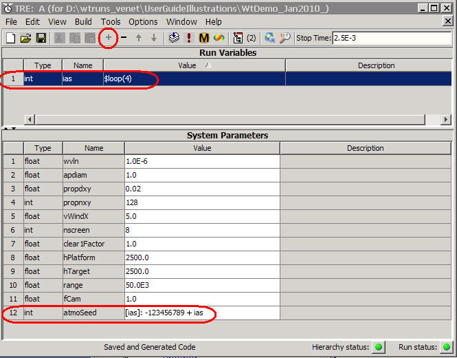
(*) Save your modified run set (File
- Save).
(*) Press the "Compile and Link" button, and then the "Execute simulation"
button as you did for your initial tutorial run.
(*) When you see from the execution
console window that execution has completed, press the TrfView button
again to inspect the results of your new *.trf file.
(If you still had TrfView open, go to its File - Open menu to
locate and open the new *.trf file).
The picture below is a screen shot of the resulting TrfView main window. Notice that you still have the same recorded variables as in the original tutorial exercise. The difference now is in the pull-down list generated by the little triangle indicated by the red arrow. As illustrated below, this now allows you to select any of four runs, corresponding to the different random number seeds discussed above. If you select a run, and then plot variable "A.simplefieldsensor.fld", you will see that the amplitude and phase maps for run 1 are identical to the results of your initial tutorial exercise, but the maps from subsequent runs have a different appearance. Note that each run still consists of three sensor exposures.
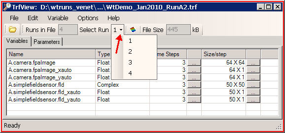
Elevating parameters and the system hierarchy
The concept of "elevating" parameters is something that you already used numerous times in the above tutorial, although we did not use the "elevating" terminology before. For example, recall the very first setting expression that you entered in the introductory tutorial: in the SimpleFieldSensor, you assigned the symbol "wvln" as the value of the parameter named "wavelength". By assigning a symbol name instead of a numerical value in the System Editor, you chose to defer the assignment of a numerical value to a higher level in the system hierarchy. In this case, SimpleFieldSensor existed at the top system level of your model, so the only higher level is the Run Set level. In WaveTrain lingo, we say that you "elevated" the parameter named "wavelength" to a higher level.
In the tutorial, you elevated numerous
parameters when you entered the setting expressions for all your components.
In the tutorial, you always accomplished this by
(i) typing a symbol name, or expression, in the value field of a
parameter, then
(ii) pressing the "Add As Parameter" button in the "Undefined Identifiers"
pop-up window (if the symbol name was a new one).
There is an alternate elevation procedure
which some WaveTrain users find convenient. If you want to elevate a
parameter, but you want the setting expression to be the same symbol that was
already used for the parameter name, then you can just
(i) right-click on the parameter name
(ii) select "Elevate" from the context menu.
If you experiment with this, you will see that this "Elevate" procedure creates
the setting expression, and registers the symbol name without popping up
the "Undefined Identifiers" window.
As you progress with WaveTrain, and create more complicated systems, you will eventually want to group sets of components into subsystems. In that case, your hierarchy will consist of the Run Set, the top-level system, and perhaps several levels of subsystems. You can elevate any parameter from any given level to any higher level, up to the Run Set level, before you assign a numerical value. This is quite important for organizing your parameters into logical and easily accessible groups. If you think that you will want to vary a parameter value from one system run to the next, then you will want to elevate that parameter to the Run Set level. That way, you can leave your system unchanged, and just change the runset in order to change parameter values.
Changing the list order of System Parameters - variable dependencies
When you finished entering the setting
expressions in your tutorial system, the symbols appeared in a certain order in
the Parameters panel of the System Editor. This original order was
simply the order in which you defined the symbols. This order is preserved
in the list that appears in System Parameters panel of the Run Set Editor
(these two parameter lists are actually the same list). The original list
order may be undesirable for two reasons:
(a) From a human-interaction (or just aesthetic) point of view, you may
want a certain grouping of symbols in the Run Set Editor: e.g., all sensor
parameters together, all source parameters together, etc.
(b) More seriously, the Run Set Editor (System Parameters panel and Run
Variables panel) has a restriction on the list order if you want to express one
value in terms of other names in the list. Because of the way entries are
parsed by the underlying code, a setting expression can only use symbols that
have been assigned values previously (above) in the list.
This restriction may require you to change the existing list order to accomplish
the linkages you want.
To learn more about changing the parameter list order, and to see further examples of how to link parameters to each other, you should consult the relevant sections of the details chapter on data entry, located later in this User Guide.
The list order discussed above is defined by the numbers in the left-most column of the Parameters panel and the left-most column of the Run Variables panel. In the Run Set Editor, you may left-click on the Name column header, which causes the names to be re-sorted alphabetically. However, as you can see, this does not change the number indices associated with the names. This alphabetic sorting does not change the list order that is relevant to the linking of setting expression discussed above.
Cleaning up in the System Parameters panel (System Editor)
Entering setting expressions in your system components will involve a certain amount of experimentation, or changing your mind about some symbol names after having already registered the names. When you are finished with your entries at your top system level, you will want to clean up by deleting names that are no longer being used. If the Parameters list contains unused names, the System Editor "System status" bulb will be yellow: if you press the bulb, you will see a report window analogous to the following illustration:
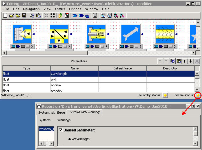
In the illustration, the report generated by pressing the status bulb (circled in red) is warning you that "wavelength" is an "unused parameter". This situation most likely occurred because, at some point in the entry of setting expressions, you accepted (registered) "wavelength" as a symbol, and then performed some later editing in which you replaced "wavelength" by a different symbol (we decided to use "wvln" in the earlier tutorial).
(*) To remove the unused parameter
symbol, select (left-click) its row in the Parameters panel, then press the
![]() button in
the small toolbar at the upper right of the Parameters panel.
button in
the small toolbar at the upper right of the Parameters panel.
(*) Excute File - Save in the System Editor window to save the
change. If you have a run set open, you may also have to perform an
Edit - Update in the Run Set Editor window to re-synchronize the run set
data.
Updating Run Set Editor after System Editor changes
Suppose that you have already created a run set for a WaveTrain system, and then you subsequently edit the system in the System Editor. Many such changes will temporarily render the run set invalid, and you must execute Edit - Update in the Run Set Editor window to continue working there. There should be no confusion as to whether you need to do this: the condition is signalled by the message "Obsolete" in the status bar at the bottom of the Run Set Editor, and by the inability to access various grayed-out menu options.
If a run set is not open when you edit its system, then the "Obsolete" message will appear when you next open the run set. There is no possibility of incorrectly executing the simulation run due to forgotting to perform this synchronization step.
Simple documentation - the "Description" fields in the Editors
In your tutorial work, you doubtless observed that the Parameters panel in the System Editor, and the Run Set Editor both have entry fields entitled "Description". These fields are available for the user to enter arbitrary documentation comments. Comments may be entered in the Parameters panel of the System Editor, and in the Run Variables panel of the Run Set Editor. The Parameters descriptions are automatically copied to the System Parameters panel in the Run Set Editor.
Note that the column widths in the Editor windows can be altered by dragging the separators in the column header labels.
Discarding recent edits
In the System Editor, you can execute the menu command Edit - Discard Changes in order to undo any changes you've made since the last Save operation. But, note there is no "undo" button that allows you to undo step by step, or going back before your last save.
Further details
For further details and a comprehensive review of data entry in the Editors, you should consult the User Guide details chapter on data entry.
After completing the above tutorial, new users will no doubt still have many questions about the usage of specific WaveTrain components, system assembly, data entry in setting expressions, and inspecting and post-processing WaveTrain results. Details of these subjects are treated in the remaining chapters of this User Guide.
After the introductory tutorial, several alternatives for further WaveTrain
learning are as follows:
(a) Users can attempt to construct their own simple systems from scratch.
(b) Users may attempt to add embellishments or make modifications in the
tutorial system, which is already a physically interesting and non-trivial
system.
(c) Users may wish to move on to study the
BLAT system, which is included in
the WaveTrain examples directory. This example system can introduce the
reader to usage of WaveTrain's adaptive-optics components. The BLAT model
is also accessible from a
link on
MZA's web site,
However users proceed, we recommend at this point that they
(a) Skim the rest of the User Guide to get a notion of the contents and
organization
(b) Dive into the details as they are needed for the user's future
WaveTrain work.
The remaining detail sections in the User Guide are grouped into the
following categories:
(*) For physics-oriented issues and usage details regarding important
specific WaveTrain library systems, users should consult the chapter
Modeling details.
(*) For details regarding data entry in the two editor windows, users
should consult the chapter Data entry in subsystem
parameters and inputs, and in the Run Set Editor.
(*) For details regarding TrfView, trf files (recorded outputs) and the
extraction of trf
data, users should consult the chapter Inspecting and
post-processing WaveTrain output: *.trf files, TrfView, and Matlab.
(*) For details regarding the construction of user-defined WaveTrain
subsystems, users should consult the chapter
Creating user-defined WaveTrain components.
Modeling details
Connecting WaveTrain components
Each WaveTrain component has inputs and outputs, and by connecting inputs to outputs we define which subsystems interact with one another, and how. Connecting the components of a WaveTrain system and setting the parameters can be performed in any order, and interspersed at will.
WaveTrain is based on tempus, a general purpose simulation tool, and in tempus a connection between two subsystems can represent any kind of interaction at all - forces, control signals, sensor outputs, message packets, whatever. Of course, in WaveTrain, many connections between components represent optical interfaces, and we designed a C++ class, WaveTrain specifically for that purpose; that is the origin of the name for the overall tool. A single connection of type WaveTrain can describe all the light crossing a given plane in a given direction, from any number of sources, coherent or incoherent, polarized or unpolarized.
Most WaveTrain subsystems have one or more inputs and/or outputs of type WaveTrain; light sources, like lasers, typically have a single WaveTrain output, while light sensors, like cameras, typically have a single WaveTrain input. Two-way optical components, like mirrors and lenses, generally have two WaveTrain inputs and two WaveTrain outputs, one of each for each propagation direction. By convention, when a component has just a single WaveTrain input it is named incident, while if it has a just a single WaveTrain output, it is called transmitted. Note that transmitted waves may correspond to physical reflection, refraction or diffraction: "transmitted" is used in a generic sense simply to indicate the wave or waves that emerge from the component in question.
The WaveTrain inputs for a two-way optical component are named incomingIncident and outgoingIncident, while the corresponding outputs are called incomingTransmitted and outgoingTransmitted. The terms "incoming" and "outgoing" are used only to distinguish between the two inputs and the two outputs, and indicate which is related to which. The effects of some components are direction-independent (e.g. Aperture) but for many components that is not true. For further details regarding WaveTrain's directional nomenclature and coordinate systems, see the section on "Spatial coordinates and direction nomenclature".
Basics of connecting inputs and outputs
Subsystem inputs can be
(a) connected to an output of some other subsystem, or
(b) assigned a setting expression (possibly by default) and left
unconnected.
It is also allowed for an input to have a setting expression and be
connected to another system's output: in that case, the output will
supersede the setting expression, if an output is available at a
particular virtual simulation instant.
In more advanced work, you will also find it useful to connect an input to an
input of the composite system that contains it.
To connect an input to an output, the procedure is very
simple:
(a) place the cursor on the arrowhead of a dark-blue output bar: the
arrowhead should turn red when you are over the sensitive region;
(b) drag to the connection triangle at the end of a light-blue input bar,
and release: a connection line will appear.
For inputs of data type WaveTrain, the default value is generally set to the value WaveTrain(), which is equivalent to saying that there is no incident light. This means that it is generally OK to leave these inputs unconnected. A typical example is when only "incoming" light exists in the system. In that case, all the outgoingIncident inputs are left unconnected. Notice that this is the situation in the system you constructed in the tutorial of the previous chapter.
In order to connect an output and input, they must have the same data type. In the system pictured above, all the connected quantities were of type WaveTrain, which you can verify by displaying the type fields. An attempt to connect incompatible data types will be automatically refused by the GUI (i.e., no connecting line will appear).
Multiple output connections
A subsystem output of data type WaveTrain may be either left unconnected, or connected to exactly one input of type WaveTrain of a different subsystem. If you attempt to connect an output of type WaveTrain to a second input, you will receive an error message. In more advanced work, you will also find it useful to connect a WaveTrain-type output to one output of type WaveTrain of the containing system.
Although you cannot connect one WaveTrain-type output to two inputs, you will frequently want to model an optical system in which the same wave or waves are seen by two or more different sensors, or sent through two or more different optical paths. The mechanism provided for this purpose is a special component called a Splitter, which has one WaveTrain input and two WaveTrain outputs. Similarly, if you want to combine the light from two or more sources and send it through the same optical path you must use another special component called a Combiner, which has two WaveTrain inputs and one WaveTrain input. All splitting and combining can be done with these, but for convenience we also provide a number of other closely-related components: IncomingSplitter, IncomingSplitter6, OutgoingSplitter, IncomingCombiner, OutgoingCombiner. For more information, see Splitting and combining optical paths.
Outputs of data type other than WaveTrain can be connected to any number of subsequent inputs, without special splitting mechanisms. Examples of such outputs are fpaImage of Camera (data type Grid<float>) and fld of SimpleFieldSensor (data type Grid<Complex>).
Managing connections and the display
As a practical matter, you will find that when making
connections it helps to have some "elbow room", enough space between subsystem
to make it easy to see what is connected to what. If the subsystem icons are
close together, when you display the subsystem inputs and outputs they will
often overlap one another, as shown, making the diagram very hard to read.
You could simply spread the subsystems further apart by dragging them, but
unless you do that only a few a time the total diagram can become too large to
fit in the window. How to proceed in this context is largely a matter of
user preference, but another mechanism is provided to help cope with space
issues. The System Editor window toolbar has two buttons whose icons are ![]() (Expand block diagram) and
(Expand block diagram) and
![]() (Pack block
diagram). Clicking on
(Pack block
diagram). Clicking on ![]() increases the distance between all subsystems by a factor of two. When we
are done making connections, we can hide the inputs and outputs if desired, and
use the pack button
increases the distance between all subsystems by a factor of two. When we
are done making connections, we can hide the inputs and outputs if desired, and
use the pack button ![]() to return to the original diagram scale. If we hide the inputs and
outputs, the connections are simply indicated by single- or double-headed arrows
between the icons:
to return to the original diagram scale. If we hide the inputs and
outputs, the connections are simply indicated by single- or double-headed arrows
between the icons:
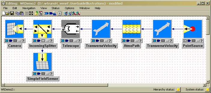
In the above diagram we have only single-headed arrows because light is only propagating in one direction in this system.
Other useful display manipulations: Particularly when we desire to leave inputs and outputs displayed, the connecting lines are often at unpleasant angles, or passing behind other icons, or generally forming a jumble that impedes the clear display of the logical connections. Two manipulations are provided to help clean up the diagram:
(a) The connection triangles or arrowheads on inputs and outputs may be flipped from one side to the other of the input or output colored bars. To do so, place the cursor on a colored bar and double-left-click. Alternatively, place the cursor on a bar and right-click to get a context-sensitive menu that offers the "Flip" option. This option is very useful for preventing the obscuration of connecting lines.
(b) If you left-click anywhere on a connecting line and drag, you will see that a new vertex is created, leaving you with a connecting polygon instead of a single line segment. This allows you to create more-horizontal or vertical connecting paths, and generally move lines so that they are more visible. Also, if you place the cursor on an existing connecting line or vertex and right-click, you will get a context-sensitive menu with related options, such as deleting a vertex.
Physical units and nomenclature
Units
Unless an explicit statement to the contrary is given, all numerical quantities used in WaveTrain are expressed in MKS (meter-kilogram-second) units, and all angles are expressed in radians. The documentation for individual library subsystems is usually explicit about the physical units for inputs, parameters and outputs. (The individual-system documentation is the html page that appears when one clicks the "?" symbol below a subsystem icon in the System Editor window). However, if a unit specification has been omitted, the user should feel confident in assuming MKS units. This applies particularly to WaveTrain data that is saved in .trf files: .trf data does not have physical units information explicitly indicated in the .trf file.
One potential ambiguity that arises is the physical unit of wavefront optical path difference (OPD). "MKS" in this case could refer either to absolute length (meters) or to radians of phase. In WaveTrain, OPD is almost always expressed in meters. The documentation of individual subsystems should be explicit in this regard.
Time in WaveTrain is always expressed in units of seconds.
Physical nomenclature
There are several important optics quantities for which no universally consistent nomenclature exists. We mention several key items here, and compare commonly used names with the names that were adopted in WaveTrain.
Irradiance, intensity: These terms are often used interchangeably for the quantity whose MKS units are W/m2. "Irradiance" is the term recommended by specialists in radiometry and by the standards committees, but the use of "intensity" has a long history in physics texts. In the WaveTrain documentation and system modules, these two terms will also appear interchangeably.
Exposure, integrated intensity: The term "exposure" is often used for the product (irradiance)*(exposure length), whose MKS units are (W/m2)*sec= J/m2. In WaveTrain modules, this quantity is almost always referred to as "integrated intensity", where "integration" in this case refers to the time dimension. "Integrated intensity" is the standard output of all WaveTrain intensity- or energy-type optical sensors.
Integrated complex field: This is an unphysical quantity which appears in at least one important WaveTrain sensor module. WaveTrain's SimpleFieldSensor module was provided to make the complex optical field directly accessible to the user. For reasons of coding uniformity with respect to the other temporally-integrating sensors, it was originally decided to define the output of the field sensor as (complex field)*(exposure length), with units of (W/m2)1/2 * (sec). Of course, physically this is not a meaningful quantity, and does not scale sensibly with exposure length.
The user must apply the appropriate scale
factor to renormalize SimpleFieldSensor's output to a physically meaningful
quantity. Suppose icf denotes SimpleFieldSensor's integrated complex field
output. Then, in order to obtain the physically sensible
integrated intensity in J/m2, one
must compute in post-processing the quantity
integrated_intensity = |icf|2 /
exposure_length .
(Note that |icf|2 / exposure_length = |c_field*exposure_length|2
/ exposure_length
= |c_field|2 * exposure_length
= integrated_intensity ).
Spatial coordinates and direction nomenclature
WaveTrain assumes that all optical beams propagate at small angles relative to the z axis. Beams may propagate in the (+z) or (-z) directions. Any physical sequence of optical components that fold or refract light through large angles (such as steering mirrors) should be visualized in terms of an unfolded path, as far as the WaveTrain model is concerned. Every WaveTrain module (subsystem) has a local (x,y,z) coordinate system, and characteristics such as aperture support and source module beam profiles are defined with respect to their respective local coordinate origins. In the absence of explicitly imposed transverse displacements, each module (subsystem) in a WaveTrain system has its local coordinate origin on the z axis of a conceptual global coordinate system. We emphasize the word conceptual, because WaveTrain does not actually assign global z coordinates: the only z distances actually input into WaveTrain are propagation distances, |Dz|, between modules. More precisely, these |Dz| are the distances between the local origins of two modules. The direction (positive or negative) associated with |Dz| is specified by "outgoing" and "incoming" tags as described below.
Propagation distances |Dz| are specified in the inputs or parameters of propagation modules such as AtmoPath or VacuumProp. As will be explained soon, it is also typical in wave-optics modeling to have many optical-system components with zero separation. Zero separation between neighboring modules is assumed, whenever no |Dz| is explicitly specified.
When constructing WaveTrain models, users must clearly understand some specialized directional nomenclature used by WaveTrain. Three key pairs of terms are used everywhere in WaveTrain with specialized meanings. These terms are "Incident/Transmitted", "Outgoing/Incoming" and "Platform/Target".
"Incident" and "Transmitted" tags
As explained above, the physical sequence of optical components modeled in WaveTrain should be visualized in terms of an unfolded path. Any beam that enters a WaveTrain module is called "Incident", and any beam that exits a module is called "Transmitted". In particular, a WaveTrain "Transmitted" beam can refer to light that was physically reflected, transmitted or internally generated (by a source). For examples of incident and transmitted tags, see the input/output bars (the light and dark blue bars) in the System Editor picture below.
"Outgoing" and "Incoming" tags: orientation of +z
Positive- and negative-z directions are defined in WaveTrain via the "outgoing" and "incoming" tags that appears in the input/output lists of various propagator and other modules. The (+z) direction is identified with the "outgoing" direction tag, and the (- z) direction is identified with the "incoming" direction tag. For example, the figure below shows two separate systems consisting of a PointSource source and a TargetBoard sensor connected via the AtmoPath module.
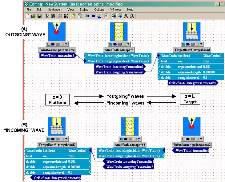
In system (A), the wave emerging from PointSource is connected to the "outgoingIncident" input of AtmoPath. Consequently, the wave traveling from PointSource to TargetBoard is defined to be traveling in the (+z) direction. Usually, it is acceptable to think of PointSource as located at z=0 and TargetBoard as located at z=+L, although this is not literally what WaveTrain does internally. As stated previously, WaveTrain only works with z differences between or across modules. The absence of an absolute 0 of z is significant if one works with a WaveTrain system that contains several (i.e, more than one) concatenated atmospheric modules. In that case, the z-coordinates of phase screens within each atmospheric module refer to relative positions within that atmospheric module only.
In system (B), the wave emerging from PointSource is connected to the "incomingIncident" input of AtmoPath. Consequently, the wave traveling from PointSource to TargetBoard is defined to be traveling in the (- z) direction. We can think of TargetBoard as located at z=0 and PointSource as located at z=+L, with the caution mentioned above. In general, both outgoing and incoming waves can be present in a single system.
The visual layout (right-left, top-bottom) of the subsystems in the System Editor has absolutely nothing to do with establishing (+z) and (-z) directions. The only thing that matters are the "outgoing" and "incoming" tags established by certain of WaveTrain's subsystems. In the above example systems (A) and (B), we positioned components so that an outgoing wave (+z) points to the right, and an incoming wave (-z) points to the left, but that was solely to help in human visualization.
In the above examples, AtmoPath provided the outgoing/incoming assignments. If AtmoPath is not included in a WaveTrain system, there will usually be some other module that establishes the assignments "outgoing" (+z) and/or "incoming" (-z). However, not all WaveTrain modules that deal with wave inputs or outputs need to designate the input/output as outgoing or incoming. For example, we see in the preceding picture that PointSource simply generates a wave designated as "transmitted", without specifying whether that means outgoing or incoming. Whether a module needs to know that a wave is outgoing or incoming depends on the mathematical operation that module will perform on the complex field.
Side remark regarding GUI manipulation: In the preceding diagram, notice that in system (A) the inputs all have their triangle connectors on the left sides of the modules, whereas in system (B) the input connectors are all on the right sides of the modules. The output connectors stand in an analogous relation. This flipping of inputs or outputs is accomplished by right-clicking on a module, and then choosing the "Flip inputs(outputs)" command (double-clicking on the input or output bar does the same thing). Flipping is not necessary to make the system function, but it greatly improves the graphical readability.
As described above, the system connections to "outgoing"
and "incoming" input/output boxes are the only determinants of positive and
negative z direction. Additionally, at many places in the WaveTrain
documentation, the terms "platform" and "target" are used in the following
specialized directional sense:
"Target" means the more-positive z end of the system
(the destination of "outgoing" waves or the source of "incoming" waves), while
"Platform" means the more-negative z end of the system
(the destination of "incoming" waves or the source of "outgoing" waves).
The user should realize that the terms "platform" and "target" never appear in any of the objects that are manipulated in WaveTrain's System Editor window. The only directional specifications that the user directly designates when building a system are "outgoing" and "incoming". "Platform" and "target" ends can both contain sources, sensors or reflectors: there is no restriction in that regard. The additional "platform-target" terminology may initially seem redundant or confusing, and may conflict with what is really the physical target of a beam in a particular application. However, this terminology is now thoroughly ingrained in WaveTrain documentation and usage.
WaveTrain's x and y axes are two Cartesian axes transverse to the z axis, where the latter is always the nominal propagation direction. There is no intrinsic relation between WaveTrain's (x,y,z) directions and any earth-connected coordinate system. There is no intrinsic association with up, down, right, left, horizontal or vertical. Each WaveTrain module has its local x-y coordinate system, and the defining characteristics of the module (e.g., aperture boundary, focus aberration curvature factor, position offset, etc.) are all defined relative to that local x-y coordinate system. The local z axes (or x-y origins) of different modules are either colinear with each other or transversely offset from each other, as determined by the insertion (or not) of a TransverseVelocity module. The important topic of transverse displacement and transverse motion is discussed in further detail in a later section.
In many WaveTrain modules, there is no explicit specification of how the defining characteristic (e.g., Aperture boundary) is offset with respect to the local x-y origin. If there is no explicit specification, the user should assume that the characteristic in question is centered with respect to the local x-y origin.
Transformation of outgoing to incoming waves
As stated previously, mirror-like deflections in WaveTrain are modeled in terms of an unfolded optical system. Typical examples would be a beam incident on a Tilt module or on a BeamSteeringMirror module. For example, if a wave is fed to the "outgoingIncident" input of a Tilt module (see panel (A) of the following diagram), then the corresponding output beam is obtained from the "outgoingTransmitted" output of the Tilt module. An incoming wave ("incomingIncident" and "incomingTransmitted" may also be controlled by the same Tilt block, as represented by the dashed arrows in (A). This models a common situation in a laser beam projection system, where the same steering mirror might affect a projected laser beam heading toward a target, as well as beacon light returning from the target. What is not allowed is the operation shown in panel (C): one may not transform the outgoing beam to an incoming beam simply by making the connections illustrated in (C).
![]()
This restriction applies to all WaveTrain modules, but there are a few specialized reflector components that may appear to transform outgoing to incoming waves (or vice-versa). Among these are the rough-reflector modules like CoherentTarget, IncoherentReflector, or PartiallyCoherentReflector. Panel (B) of the above figure illustrates this idea. The decision to connect CoherentTarget's "transmitted" output to AtmoPath's "incomingIncident" input seems logical, since most often we want the reflected ("transmitted" in WaveTrain terminology) beam from this component to propagate back in the opposite direction through the same atmospheric screens that the incident beam saw (possibly displaced in x or y, of course). Thus, CoherentTarget and similar modules have the apparent capability of transforming {outgoing ↔ incoming}. However, what such modules are really doing is acting as both "sensors" and "sources": one should think of the module's "transmitted" wavetrain as being a new wavetrain that was generated by a source. Therefore, this type of module's "transmitted" wavetrain can be connected to either a subsequent "incoming" or "outgoing" tag. For example, if the CoherentTarget in panel (B) was meant to model a transmissive ground-glass plate, with subsequent propagation through a second atmospheric path, then it would make sense to add a second AtmoPath module to the right of CoherentTarget, and to connect CoherentTarget's "transmitted" output to the "outgoingIncident" input of that second AtmoPath.
The optical quantities that we model using WaveTrain are usually described analytically in terms of continuum (x,y,z) coordinates. For computer modeling we must represent a continuum quantity by a sampled function on a discrete lattice, or mesh of points.
Nomenclature note: the term "grid" is often used in the general literature in a sense equivalent to "lattice" or "mesh". However, in WaveTrain the term "grid" has been appropriated to designate a data type that comprises the combination of a mesh of points together with function values defined on that mesh. We will attempt to maintain consistent terminology in the documentation: we will try to use "mesh" or "lattice" when we mean just a mesh of points, and to reserve "grid" for its specialized WaveTrain meaning.
Grid spacing, dimension and offset
In the present section, we introduce several important facts about the WaveTrain meshes used for physical (Fresnel) propagation, for phase screens, for detector sample points and other purposes. Later sections of the User Guide provide further details and sample usages, in the context of specific WaveTrain subsystems or of specific functions used to define meshes. The purpose of the present section is to gather in one place some general properties of and key facts about the WaveTrain meshes. Almost all the meshes used in WaveTrain are uniform rectangular meshes aligned with the x and y axes. The dx and dy spacings and the nx and ny dimensions may be allowed to differ, although for many applications equal x and y parameters are appropriate.
There are several variations in the data entry format, but WaveTrain meshes are almost always specified in terms of the parameter set (nx, ny, dx, dy), or a notation like (nxy, dxy) to specify a square mesh using just two parameters. In the following discussion we will use the notation (x, nx, dx) for brevity to refer to either dimension. In addition to (nx,dx), the remaining specification required to completely determine the mesh coordinates is the offset from x=0. The offset determination can be somewhat confusing in Wavetrain, so we now discuss this in some detail.
Most situations can be satisfactorily modeled with two options: either the mesh is forced to have a point at x=0 or the mesh is symmetrically disposed with respect to x=0. At the WaveTrain code level, these mesh types are constructed using functions named "gwoom" (= "grid_with_origin_on_mesh") and "GridGeometry". The two examples in the following diagram define the offset convention for the case nx = even:
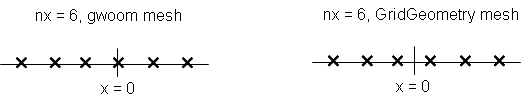
The key rules for nx = even are:
(1) In the gwoom mesh, the nxy/2 point (counting from 0) lies at x=0.
(2) In the GridGeometry mesh, the points are symmetrically positioned relative
to x=0.
The following two examples define the offset convention for the case nx = odd:
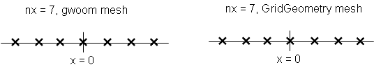
Note that when nx = odd, the two mesh-defining functions produce identical meshes.
The WaveTrain user is not always allowed to choose whether a gwoom or GridGeometry mesh will be used. In many WaveTrain library modules, the user is simply asked to enter (nx,dx), but is not asked to specify whether a gwoom or GridGeometry mesh should be used. In such cases, the mesh type will be a gwoom, unless module documentation explicitly specifies otherwise. As an example, consider the TargetBoard system in the left panel of the following picture. The parameter list calls for the specification nxy with no option to specify the grid type: this will be a gwoom mesh. The same situation holds for the sensor meshes in the SimpleFieldSensor and Camera sensors. An exception to the more common pattern is the HartmannWfsDft sensor module: again the user is just allowed to specify (nx,dx) parameters in the sensor plane, but this time a GridGeometry type of mesh is used.
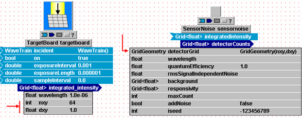
In other library modules, the user is allowed to specify the choice of gwoom or GridGeometry in addition to the (nx,dx) specification. An example is the SensorNoise block shown in the right-hand panel of the above figure. In this case, the data type of the input parameter (left-most column) is itself named GridGeometry: that is the signal that the user must enter a setting expression in the value field (right-most column) which is written in terms of either the function gwoom(...) or the function GridGeometry(...). An example using the GridGeometry function is shown in the figure. Further details of the allowed input syntax for gwoom(...) and GridGeometry(...) is given in the User Guide chapter on data entry.
New feature as of WaveTrain 2010A: To help the user verify exactly what the mesh-point coordinates were in a WaveTrain run, a new feature has been added as of WaveTrain 2010A. For all recorded variables of WaveTrain type "Grid", WaveTrain automatically saves companion recorded variables that record the mesh-coordinate information.
Propagation mesh
The propagation mesh, i.e, the mesh on which Fresnel propagation calculations are performed, has some special restrictions. This mesh is specified in PropagationController, AtmoPath, or analogous subsystems. In order to use highly optimized FFT (Fast Fourier Transform) routines, WaveTrain requires that nx for a propagation mesh be a power of 2. (Even if the user enters a non-power-of-2, WaveTrain will round up to the nearest power.)
In addition to the power-of-2 restriction, there are other constraints on the propagation mesh (nx, dx) that should be observed in order to avoid DFT (Discrete Fourier Transform) aliasing and wrap-around effects. These issues are discussed in a separate section. The propagation mesh is a gwoom, unless explicitly specification to the contrary is allowed in a propagation module.
Phase screen mesh
The mesh on which phase screens are defined is specified in AtmoPath, GeneralAtmosphere or analogous modules. To allow for relative transverse motion of the screens, sources and sensors, without repeating the screens, one may specify screens that are much longer in one dimension than another. The screens are also computed using FFT routines, but there is no power-of-2 constraint in this case. The screens must only be computed once, at the beginning of a WaveTrain run, so it is acceptable to be non-optimally efficient here. Another slight difference in the way phase screen meshes are specified is this: the spacing dx is still an input parameter, but instead of nx the user must specify the span of the screen in meters.
Further explanation of the phase mesh specifications, and how these interact with the transverse motion specifications, is deferred to a separate section.
Interpolation
When one WaveTrain module operates on the discrete complex field or other output of the preceding module, it is often necessary to interpolate the preceding output onto the mesh of the current module. This is frequently necessary even if we set those mesh items under our direct control so that the meshes are registered as much as possible. For example, suppose we have a simple static system consisting of a source, an AtmoPath module, and a TargetBoard sensor. In this case, (nx,dx) specs are requested in AtmoPath to define the propagation mesh and phase screen mesh, and in TargetBoard to define the points at which the final irradiance will be sampled. Since all these meshes are gwooms as described above, if we specify a common dx value then the mesh points of all the modules coincide and no interpolation is necessary. However, if we introduce any relative displacement in the system, such as wind, target motion or just static displacements, then it will frequently happen that the displacement for a simulation time step is not a whole number of mesh points. In that case, WaveTrain must internally interpolate to pass the optical data from some modules to others. No special action is required by the user to effect this: WaveTrain takes care of this matter internally. However, the user should be aware that interpolation is frequently occurring, because there are occasionally surprising artifacts that arise from the interpolation. These artifacts are more likely to occur when the complex field must be interpolated as opposed to a real irradiance map.
Modeling of optical systems in "object space"
The subsystems of a WaveTrain model can typically be grouped into functional groups that represent either propagation channels or optical system groups. The latter might represent transmitters, targets, or receivers. The optical system groups share one critical characteristic: it is often desirable, in wave-optics modeling, to ignore physical propagation between the components of an optical system group. All the components of a single optical system group can be modeled as operating in a space of common transverse magnification, which is usually taken as having the same transverse scale as the propagation channel. Equivalently, this transverse scale would correspond to the entrance pupil in case of a pure receiver or the exit pupil in case of a pure transmitter. For brevity in this documentation we refer to this space as the "object" space. In this modeling approach, which considerably simplifies the model bookkeeping, we specify the parameters of each optical component transversely scaled to the object space, and we usually place all the optical components in a common z plane, with zero separation between the components. In this approach, the optical system component parameters are immediately related to the turbulence and propagation parameters of the propagation medium. A wide variety of phase and amplitude map manipulation, beam splitting, detection processes and adaptive-optics feedback loops can still be accurately modeled in such a collapsed model of the optical system. The order of operations carried out by various elements (splitting, attenuating, tilting, sensing, etc.) corresponds to the order in which the WaveTrain blocks are connected, and this must be consistent with the actual order in the physical system. With one exception, in most WaveTrain modeling there is no reason to carry out physical-optics propagation using Fresnel propagators within the optical system. The one exception is computation of the far-field image in (or near) a focal plane, which is carried out in WaveTrain's Camera and HartmannWfsDft (wavefront sensor) modules. In these special case, the diffractive effects of the entrance pupil are accounted for by far-field propagations embedded in the modules. Defocused sensor planes can be accounted for as well in this framework. The omission of diffractive propagation between most elements of the optical system is consistent with the usual optical analysis of composite systems: the effects of diffraction are for practical purposes completely represented by one physical propagation from pupil to sensor plane.
The following figure shows a simple detector system that illustrates the above points.
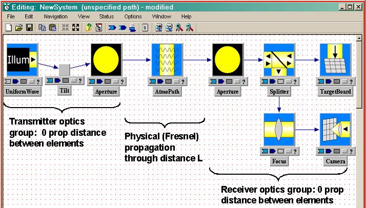
Consider the receiver optics group. Within this group, there are no subsystem inputs or parameters that specify separations between any of the subsystems. Consider first the receiver actions comprising truncation by Aperture, "splitting" or more accurately "copying" of the beam by Splitter, discrete sampling on a sensor mesh by TargetBoard, and the application of a quadratic phase by Focus. All these mathematical operations are applied to the incident complex field in the same z-plane, namely the z-plane of the aperture. The order of the operations is faithful to the connection arrows in the picture. Now the physical system that is being modeled will of course have non-0 separations between the receiver elements, and may in fact include various reimaging and demagnification stages. For example, the targetboard may model a CCD sensor on which is physically impinging a demagnified image of the physical aperture plane. As long as diffractive effects due to the reimaging optics are negligible, accurate modeling can be done by projecting the mesh spacing of the physical CCD sensor to the aperture plane. This projection to the "object space" is the usual way that optical systems (both transmitters and receivers) are simplified for modeling in WaveTrain (or any other wave-optics code) .
The Camera module in the receiver group does internally incorporate a key physical propagation. The action of Camera is to compute the diffractive far-field (Fraunhofer) irradiance corresponding to whatever input complex field is presented to Camera. In this case, diffraction by the receiver group's Aperture has a dominant effect on the irradiance distribution in the Camera sensor plane, and this diffraction is completely accounted for by the internal computations of Camera. The particular combination of geometric and physical (diffractive) propagation outlined here is very typical in the analysis and numerical modeling of optical systems. If the combination of projections to object space plus far-field Cameras is insufficient to accurately model a given optical system, then it is possible to construct a system that actually computes physical propagations between numerous optical elements. The key difficulty is properly generating the widely varying propagation mesh spacing required as the optical beam undergoes a sequence of possibly large compressions or expansions. This will usually require understanding and use of the "spherical reference wave" feature of WaveTrain's Fresnel propagator modules.
Side remark: The Focus system in the above receiver group illustrates a secondary point. A typical application of Focus in a receiver group is to allow a Camera focal plane to be the image plane conjugate to a finite (rather than infinite) distance. The composite WaveTrain module called Telescope may also be used for this purpose. See "Using the Camera module" for further discussion.
Complete systems with 0 total propagation distance
For testing purposes, it is often very useful to construct a complete WaveTrain system that has no propagation distance anywhere in the system (except possibly inside a Camera module). The only caution to be observed here is that one must be careful to actually specify the mesh on which the optical field is defined. In a typical WaveTrain system this might be accomplished by the propnxy and propdxy parameters in the AtmoPath subsystem. However, in the absence of any propagator module, the recommended procedure is to insert a PropagationController subsystem to define the mesh parameters on which the optical field is generated. Normally, one or more PropagationControllers are automatically present because they are subsystems of propagation modules such as AtmoPath. See the section devoted to PropagationControllers for further discussion.
The following figure shows an example of a complete system with 0 total propagation distance: the system tests the operation of a wavefront sensor by presenting it with a perfect plane wave of variable tilt and focus.
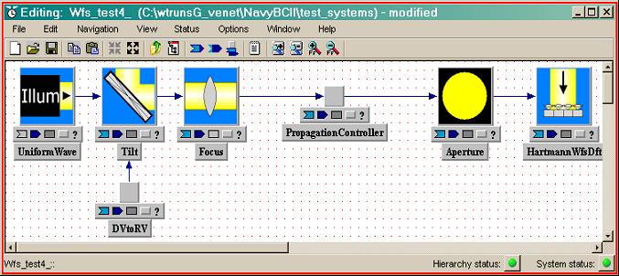
Note that WaveTrain sources such as UniformWave and GaussianCwLaser make sense when the total propagation distance is 0, but the action of WaveTrain's PointSource is ill-defined if we have no propagation distance.
Sign and phasor conventions for tilt, focus, and general OPD
There are two (linked) aspects of sign and phasor conventions that may be important to the user:
(1) For WaveTrain input purposes, the most important issue is whether positive or negative signs of tilt parameters cause beams to be deflected up or down, and whether positive or negative signs of focus parameters cause beams to converge or diverge. This is defined in the first section below ("sign conventions").
(2) A secondary issue is how signs are defined in phasor expressions that mathematically represent tilt, focus, or general transverse OPD. When defining WaveTrain inputs and parameters, the user does not usually need to know these details. However, if recorded outputs of the SimpleFieldSensor module are used to inspect complex fields, then the user may wish to know all the sign conventions used by WaveTrain for the phasors. This is discussed in the second section below ("phasor conventions").
In reading the documentation on sign and phase conventions, we recommend that the user first focus on the essential issue number (1), and just refer back to the explanations of issue (2) as needed.
Sign conventions for tilt, focus, and general OPD
Tilt
WaveTrain has several modules (notably
Tilt,
Slew
and BeamSteeringMirror)
that apply a tilt-angle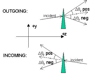 increment to an incident wave. In these modules, one inputs a tilt angle (Dqx,Dqy),
in units of radians of angle. The sign convention for tilt angle in
WaveTrain is motivated by the geometric picture of beam deflection as shown in
the following figure. The picture is drawn in unfolded form as if
deflection is effected by a prism, in accordance with WaveTrain's
"incident-transmitted" treatment of waves as discussed above.
increment to an incident wave. In these modules, one inputs a tilt angle (Dqx,Dqy),
in units of radians of angle. The sign convention for tilt angle in
WaveTrain is motivated by the geometric picture of beam deflection as shown in
the following figure. The picture is drawn in unfolded form as if
deflection is effected by a prism, in accordance with WaveTrain's
"incident-transmitted" treatment of waves as discussed above.
The diagram shows the meaning of the tilt sign when combined with the two possible z-directions of propagation. The rule is:
(a) Positive Dqy
means that the beam is steered towards positive y.
(b) Negative Dqy
means that the beam is steered towards negative y.
(c) Statements (a) and (b) hold for both outgoing and incoming
incident waves. This is consistent with the fact that, if outgoing and
incoming beams are affected by the same element, then they are both steered
toward -y or both toward +y. The interpretation of
Dqx
of course follows the identical pattern.
The representation of tilt in
WaveTrain has a twist that users must understand to work effectively.
Tilts applied by modules like Tilt
and BeamSteeringMirror
can either be
(1) carried separately in computation from the residual complex field, or
(2) incorporated into the complex field, by multiplying the incident field by a
phasor factor.
At present, we only alert the reader to the existence of this feature: the
reasons for and various implications of this dual representation are quite
important, and are discussed more fully in a later section that discusses
how tilt is modeled internally.
Focus
WaveTrain's Focus module applies a quadratic phase increment (a focus or defocus) to an incident wave. The Focus module requires a signed input value called "focusDistance", for which we here used the symbol f. The WaveTrain sign convention for focusDistance is:
(a) Positive f causes the incident wave to become more convergent.
(b) Negative f causes the incident wave to become more divergent.
(c) Statements (a) and (b) hold for both outgoing and incoming
incident waves.
The sign convention for f corresponds to what is called "power" in first-order optical design: positive power or f tends to converge an incident wave, and negative power or f tends to diverge an incident wave, regardless of the propagation direction.
Phasor conventions for tilt, focus, and general OPD
As noted in the introduction to the previous section on signs, WaveTrain's internal phasor conventions are only significant to users when they wish to inspect the complex field output of the SimpleFieldSensor module.
Tilt
If a tilt-generating module is instructed to "put the tilt into the complex field" (see the section on how tilt is modeled), then the complex field incident on the module is multiplied by the phasor
OUTGOING waves: exp[ +i(2p/l)(Dqx
x + Dqy y)
]
INCOMING waves: exp[ -i(2p/l)(Dqx
x + Dqy y)
] ,
where we recall from above that
Dqx
and Dqy may
themselves be positive or negative.
The critical reader may question the consistency of WaveTrain's tilt-angle phasor convention. For the purpose of background understanding, consider the following. Suppose we write the fundamental vectorial representation of a plane wave phasor using the "-iwt" convention:
exp[ i(k*r - wt) ] = exp[ i(kxx + kyy + kzz - wt) ] ,
where the bold quantities indicate vectors, k is the wave vector and w is the optical angular frequency. The relevant point here is this: as t advances, positive kz forces a constant-phase surface to move toward +z (what we call "outgoing"), while negative kz forces a constant-phase surface to move toward -z ("incoming"). Likewise, regardless of the sign of kz, the sign of ky determines whether the wave moves upward or downward along y, and similarly for x. Now it would be logical to define the tilt angle via the relation ky = (2p/l)(Dqy), that is, to assign the same sign to ky and to Dqy. However, we see that the WaveTrain tilt-phasor convention violates this relation, since an extra (+/-) factor has been inserted depending on (outgoing/incoming) status. The WaveTrain convention evidently conflicts with the exp[i(k*r - wt)] representation; in fact the WaveTrain convention can be viewed as switching between "-iwt" and "+iwt" conventions depending on whether outgoing or incoming waves are being represented. Nevertheless, no contradictions arise within the allowed operations of WaveTrain. Certain signs in the propagators are defined consistently with the wave phasor signs. Additionally, a critical fact is that WaveTrain's splitter/combiner modules never allow outgoing and incoming waves to be combined for possible complex superposition on a field sensor. It is only possible to compute the complex superposition of several outgoing or of several incoming waves. Under this restriction, the WaveTrain conventions will give correct interference results.
Focus
WaveTrain's Focus module applies a quadratic phase increment (a focus or defocus) to an incident wave. The complex field incident on Focus is multiplied by the phasor
OUTGOING waves: exp[ - i(2p/l)
(x2 + y2)/(2f)
]
INCOMING waves:
exp[ +i(2p/l)
(x2 + y2)/(2f)
] ,
where f is a signed input value called "focusDistance" in the Focus module. As discussed in the previous section, the sign convention for f is:
positive f causes the incident wave to become more
convergent,
negative f causes the incident wave to become more
divergent,
where this holds for both outgoing and incoming
incident waves.
WaveTrain's focus phasor sign convention has a consistency issue analogous to that discussed in the preceding tilt section. But as outlined there, no contradictions arise within the presently allowed operations of WaveTrain.
General OPD
A general, transversely-varying phase function can be represented by
f(x,y) or (2p/l)d(x,y)
where the transverse OPD function is in radians of phase (f) or in meters (d). WaveTrain has several modules (e.g., OpdMap and FixedOpdMap) which allow the multiplication of an incident wave (complex field) by a phasor created from a discrete input array d(xi, yj). The phasor factor is defined as
OUTGOING waves: exp[ +i(2p/l)d(x,y)
]
INCOMING waves:
exp[ - i(2p/l)d(x,y)
] .
For example, in light of the previous focus discussion, an input { d(xi, yj) = - |a| yj2 } should generate a phasor factor that adds a positive-f (converging) cylinder focus factor to both outgoing and incoming waves.
Absolute phase
WaveTrain does not keep track of absolute phase in its propagation modules. That is, a complete Fresnel propagation operator from plane 1 to plane 2 includes a factor exp[i(2p/l)Dz21], but this factor is omitted in WaveTrain propagations.
All sensors in WaveTrain are temporally-gated integrating sensors. For any simulation, the user specifies a sequence of exposure windows during which a sensor will accumulate light, and this sequence is the key specification that controls the number of propagation calculations that is performed during the simulation run. Successful setup of a WaveTrain simulation requires understanding of several peculiarities of the WaveTrain timing system.
The sensor exposure windows are specified by a combination of two types of inputs:
(1) Sensor
modules like TargetBoard,
Camera, or
SimpleFieldSensor
all have a set of inputs named "on", "exposureInterval", and "exposureLength".
The "exposureLength" is the length (in seconds) of a single exposure window, and
the "exposureInterval" is the time interval (in seconds) between the start of
successive exposure windows.
CAUTION: most sensors also have an additional input named
"sampleInterval", which has a
different meaning
than "exposureInterval".
(2) An output of the module called SquareWave can be connected to the "on" input of a sensor, to control the start time of the exposure window sequence.
The inputs "exposureInterval" and "exposureLength" define the underlying periodicity of a sensor's exposure scheduling. The parameters of SquareWave control the start time of the first active exposure window, and can also be used to modulate the underlying gate window repetition sequence. The meaning of modulation in this context is illustrated in example 2 below. If no SquareWave trigger module is attached to the sensor, then the sensor's "on" input must have its value set to "true" to activate the sensor. In that case, the first active exposure window starts at time t=0.
With an exception to be explained below, WaveTrain only works with time values t >=0. A simulation run always formally begins at t=0, but propagations only occur at those times and intervals required to produce the specified sensor exposures. WaveTrain operates in "event-driven" fashion, so if there are long time gaps between events there is no impact on wall-clock execution time.
Propagation delay
WaveTrain accounts for time-of-flight delay in the propagation of light. Suppose a user's timing parameters specify that a sensor exposure window opens at time tk. If the z-distance from source to sensor is L, and the speed of light is c, then a wavefront would have to leave the source at time tk' = tk -(L/c) in order to arrive at the sensor at tk. Depending on L and tk, it is possible that tk' is negative. What happens in that case depends on how the source module was coded. WaveTrain source modules are not consistent in this regard: some are capable of answering a "request" for emission prior to t=0, but others are not. In order to avoid surprises, we recommend that the user define sensor and trigger inputs so that no exposure windows require light that must be emitted prior to t=0. However, violating this guideline is usually not catastrophic: the sensor may simply report 0 output for those exposure windows that need emissions prior to t=0.
Integration over one "exposureLength", and number of propagations in one "exposureLength"
We stated above that WaveTrain sensors are "integrating" sensors. Now we discuss more precisely what this means in WaveTrain.
The default behavior of sensors is as follows.
If an exposure window opens at tk, then:
(1) A wavefront is generated at the source at the advanced time tk'
, and this wavefront is propagated with physical delays through the intermediate
system planes. (These intermediate planes might, e.g., contain moving
phase screens, each of which will be positioned at its appropriate transverse
locations as the wavefront reaches it).
(2) If "exposureLength"=Texp, then at tkout
= tk+Texp , an intensity sensor will report an output
value defined by output = (sensor irradiance in W/m2)*(Texp)
= (exposure in J/m2). The nomenclature that was adopted in
WaveTrain uses the term "integrated intensity" for the quantity whose units are
J/m2.
Note that the default integration procedure defined in the preceding paragraph (2) assumes that the irradiance at the sensor remains constant during "exposureLength". Note also that the default procedure requires only one propagation series for each exposure window. A propagation series refers to the set of propagations and phasor multiplications that are needed to propagate one wavefront from a source, through all phase screens and optics, to a sensor.
If the default integration procedure is not acceptable for the modeling task in question, then an optional sensor behavior can be invoked by explicitly setting the input named "sampleInterval", which appears in all the sensor modules. The default setting is 0.0, which produces the default integration behavior defined above. Changing the setting to a non-0 value (but smaller than Texp) causes WaveTrain to subdivide each exposure window and propagate several wavefronts, at intervals of "sampleInterval". The individual sensor irradiances are then multiplied by sampleInterval and added, thereby still yielding a single reported exposure (integrated intensity) for a given exposure window.
When output from a sensor is recorded in a .trf file, the .trf file contains a vector of times and a corresponding set of exposure maps, one map for each time. The recorded times are the ends of the exposure windows, denoted above as tkout. The logic for recording the end times is that they represent the times when the outputs are actually available from the physical sensor. In fact, some sensor modules have an optional processing delay parameter (e.g., see Camera). In that case, the recorded .trf times are the ends of the exposure windows plus the processing lag.
Example 1
Consider the following WaveTrain system:
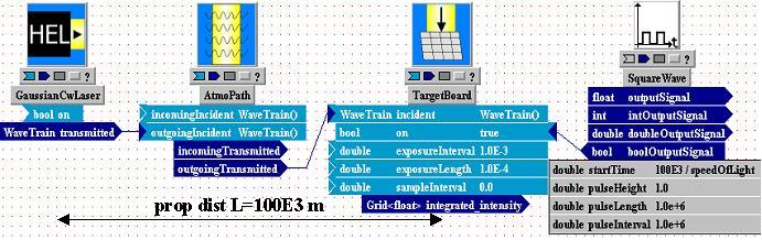
The propagation distance L=100km has been specified in the
AtmoPath module. The
SquareWave bool-type output is connected to (and triggers) the TargetBoard
bool-type input named "on".
The SquareWave timing parameters are
startTime = 100E3 m / speedOfLight (the constant
speedOfLight is an internally
defined symbol in WaveTrain)
pulseLength = 1.0E6 sec
pulseInterval = 1.0E6 sec
The TargetBoard timing parameters are
exposureInterval = 1.0E-3 sec
exposureLength = 1.0E-4 sec
sampleInterval = 0.0
Suppose also that the simulation stopTime (specified in the Run Set
editor) is 3.0E-3 sec.
The specified SquareWave startTime defines the beginning of the first sensor exposure window, and exposureInterval defines the interval between the beginning of successive exposures. Given the simulation stopTime, the following diagram shows the three exposure windows for which propagations will be generated by the above timing specifications. The exposure windows defined by the TargetBoard parameters are indicated by thin black lines, the SquareWave timing pulse is indicated by the heavier green lines, and the simulation Stop Time is the heavy black line:
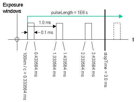
Since sampleInterval was 0.0, one propagation series will occur for each exposure window, timed so that the wavefront arrives at the sensor at the beginning of the corresponding window.
Notice that the sensor startTime of (100km)/(speedOfLight) means that the wavefront that arrives at the sensor at startTime must be generated by the source exactly at t=0. This is not a requirement for the emission of the first wavefront of the simulation: any time >= 0 is always acceptable.
In the Example 1 system diagram, we entered the timing parameters as numerical values in the value fields of the subsystem blocks. However, we would often prefer to enter variables in the value fields, and elevate these variables to the level of the Run Set editor before assigning specific numbers.
In Example 1, SquareWave's pulseLength and pulseInterval have no effect because they extend beyond the simulation stopTime. Example 2 shows how these parameters can be used to modulate the timing pattern.
Example 2
The following diagram shows how the SquareWave pulseLength and pulseInterval can be used to modulate the sequence of sensor exposure windows that are active. The active exposure windows are those that fall during the high part of the SquareWave signal. The demand for such timing sequences is not particularly high in WaveTrain practice, but the following special case is often useful. We may often include a diagnostic sensor in a system, and it may be sufficient to record just a few data frames at the beginning or perhaps the end of the simulation run. Suitable combinations of startTime, pulseLength and pulseInterval can conveniently achieve this. Note that a pulseInterval or a pulseLength that extends beyond the stopTIme of the simulation is a legal specification (this feature was already used in Example 1). The simulation stopTime, specified in the Run Set editor, always cuts off the simulation at that designated instant.
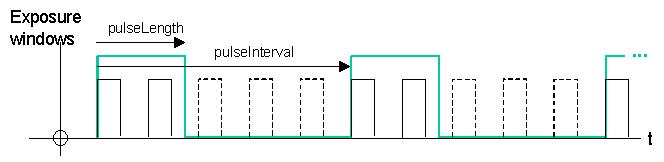
Sensor timing, CW sources and pulsed sources
In the above discussion of sensor timing
and triggering, we implicitly assumed that the WaveTrain source modules were
of the continuous-wave (CW) type. Of course as a numerical code WaveTrain
only computes wavefronts at discrete instants. The meaning of "CW" here is
that a CW source can emit a wavefront
whenever required by the sensor timing and triggering
parameters. Key CW sources in WaveTrain are
UniformWave,
GaussianCwLaser
and PointSource. In
previous discussion of sensors and timing, we noted two key facts:
(1) setting sensor timing parameters causes the so-called CW sources to
emit a wavefront at corresponding discrete times (accounting for propagation
delay);
(2) sensor output is always a temporally-integrated quantity (such as J/m2),
over a sensor exposureLength.
From these two facts, it follows that a pulsed source can be easily represented
by WaveTrain's so-called "CW" sources. We need only specify the correct
combination of source strength and sensor exposureLength, so that the total
energy emitted by the source during exposureLength is the desired pulse energy.
This technique is an important alternative in WaveTrain to the use of an
explicitly pulsed source (it may be, for example, that a source module with
desired characteristics does not exist in pulsed form).
Nevertheless, WaveTrain does provide a number of source modules that, in certain respects, explicitly represent physically pulsed sources. An example is the module PulsedPointSource. The module names can unfortunately be a bit confusing, because (1) the names of the pulsed-source modules do not always parallel the CW modules, and (2) the names sometimes but not always contain the word "Pulsed" (just as CW sources only sometimes contain the word "CW") . The user should scan SourceLib for the current list of available modules.
When a pulsed source module is used, the user must still set up sensor timing and triggering parameters exactly as explained in connection with the CW sources. The only really new feature is that timing parameters may be specified so that a source pulse may not be entirely contained within an exposure window. The pulsed-source modules are not designed to accurately model various temporal envelopes of pulses. In all pulsed-source modules, the intensity profile of each pulse is modeled as triangular in time, and symmetric. For example, the intensity of a one-microsecond pulse rises linearly from zero to its peak over the first half microsecond, then falls linearly to zero over the second half microsecond. As long as the entire pulse falls within the exposure window, all of its energy will be deposited on the detector. If a pulse arrival should overlap the beginning or end of an exposure window, only the corresponding portion of its energy will be detected (based on area under the triangle envelope). If no part of a pulse overlaps an exposure window for a given sensor, then the sensor will report zero energy for that exposure window.
Pulsed sources all contain a pair of parameters named
"pulseInterval" and "pulseLength", and an input named "on". (For an
example, see
PulsedPointSource). The meaning of "pulseInterval" and "pulseLength"
is self-explanatory. The input "on" has the same triggering functionality
as the "on" input in sensor modules. That is, "on" can either:
(1) be assigned the value "true", which turns the source on at t=0, or
(2) be connected to a
SquareWave
module, which can then be set to trigger the first source pulse at an arbitrary
start time. The section on sensor timing and triggering
illustrates more fully the use of SquareWave for triggering. The
triggering principles are the same whether applied to sensors or pulsed sources.
Although the extra functionality provided by the pulsed-source modeling is fairly restricted, the user may find it a convenient way to explicitly model the time multiplexing in physical source systems. The user should be aware, though, that this can always be done with WaveTrain's CW sources. Pulse energy can be represented as discussed in the introductory paragraph, and some adjunct procedures can be used to control which sensors see which sources. These adjunct methods include spectral filters and "polarization" tags. The use of "polarization" tags in WaveTrain is discussed in using Polarizers to separate light from different sources. We put "polarization" in quotes here because in WaveTrain the specified polarization state is just a numerical tag that allows one to differentiate two beams of the same wavelength. The main point we want to emphasize is that the choice between using a CW or a pulsed source is generally a matter of user experience or procedural preference, rather than strict WaveTrain necessity.
Transverse (x,y) displacement and motion (TransverseVelocity and Slew)
A variety of interesting WaveTrain simulation studies can
be performed without explicitly modeling any relative motion of the subsystems.
This type of simulation has the following structure:
(1) Using one value of a random number seed, define one realization of a
sequence of phase screens between source(s) and sensor(s). The seed would
be entered, for example, in the
AtmoPath module.
(2) Propagate the optical beam(s) to obtain one statistical
realization of the field(s) at all sensors. This constitutes
one "run", as recorded in the .trf file.
(3) Using the looping capability in the Run
Set Editor, change the random number seed and generate a new (independent)
realization of the sequence of phase screens, and propagate the optical beam(s)
once more.
(4) Repeat N times.
This type of simulation produces N statistically independent sample results from
each sensor, and is useful for certain types of statistical studies of
turbulence effects.
Side remark: In the above type of statistical study, the simulation Stop Time parameter should be set so that only one sensor exposure is recorded for any run, given the exposureInterval of the sensor. Otherwise, one "run" in the .trf file will contain identical repetitions of the sensor results for a given screen set realization. The duplicate results would all be correct, but execution time and storage would be wasted.
Although the type of statistical study described above is important, a more general scenario involves simulating the relative transverse motion of subsystems, while sampling the optical beams at specified rates. The key modeling assumption is that the phase screens, which are generated at the beginning of a run, move relative to sources and sensors according to the frozen-flow concept. Any study that involves rates of temporal evolution, such as calculation of the effectiveness of turbulence compensation and adaptive optics, is of this type. In such studies, the WaveTrain system must contain one or more subsystems that define relative motion between various parts of the system. In this case, one "run" of the simulation, as defined by the recorded .trf data, consists of sensor results for a designated number of time steps. The number of time steps is determined by sampling rates defined in sensor subsystems together with the simulation Stop Time. The entire simulation may consist of only one "run" that lasts the designated time. Alternatively, using the loop capability in the Run Set Editor, the entire simulation may consist of several statistically independent runs of the same temporal length, that differ only in the seed used to generate the phase screens set. For any given run, a given phase screen set is generated, and subsequently the appropriate translations cause the optical beams to interact with different portions of the screens as the subsystem positions evolve in time.
As discussed in the preceding sections on sensor timing, WaveTrain always makes use of the concept of propagation delay (finite light speed) when computing the optical field that impinges on a sensor at any time t. This has a number of consequences when we construct WaveTrain systems and define parameters that specify transverse motion. The following sections discuss in detail how transverse motion is specified in WaveTrain, and how one handles the related effects of propagation delay.
Methods of implementing relative transverse motion
WaveTrain provides the following procedures for specifying the relative motion of sources, sensors and turbulent medium:
(1) The WaveTrain module TransverseVelocity specifies a transverse offset between modules located on the negative-z and positive-z sides (incoming and outgoing sides) of TransverseVelocity. The transverse offset may be static or time-varying. TransverseVelocity blocks can be used to model uniformly moving platforms and/or targets, and/or a uniform atmospheric wind. Some examples and details of TransverseVelocity and Slew usage are given below.
(2) Frequently, it is also necessary to use a Slew module in conjunction with TransverseVelocity, in order to keep beam(s) centered on sensor entrance pupils, and to keep focal spots at a fixed field angle on camera focal planes. This corresponds physically to tilting a transmitter or receiver system in order to stay pointed at the nominal position of a target or source. However, the need for Slew depends on the type of source and sensor being used.
(3) When a TransverseVelocity block is present, WaveTrain internally computes the implied relative displacement of each phase screen and any propagating beams. But in addition, extra transverse velocities may be explicitly assigned to the individual phase screens by using input arguments in the AcsAtmSpec function. AcsAtmSpec is typically used in a setting expression in AtmoPath or similar modules. The velocities entered in AcsAtmSpec are usually reserved to represent a true atmospheric wind which varies along the propagation path. As noted in paragraph (1), a uniform atmospheric wind can be modeled using just the TransverseVelocity modules.
The combination of procedures (1), (2) and (3) allows the WaveTrain user to input rather general motion specifications for platform, target and true atmospheric wind in a natural way. By "natural", we mean that target and platform velocities would be specified in TransverseVelocity modules, and true atmospheric wind velocities would be entered as arguments of AcsAtmSpec in AtmoPath or analogous modules. As noted above, in the special case where the true atmospheric wind is uniform, it may be easier to combine the true wind with the platform and target velocities in TransverseVelocity blocks. Examples below will illustrate this. Another alternative, if the user wishes to exercise it, is to manually calculate the net pseudo-wind velocity that characterizes the motion of each phase screen relative to the beam(s). Algebraic expressions for these velocities could then be applied to the screens in AcsAtmSpec, and one could dispense with the TransverseVelocity module completely. This is a common procedure in wave-optics simulation, but in the WaveTrain world the usual practice is to use the combination of methods (1), (2) and (3) outlined above.
The principal restriction on WaveTrain motion specifications is uniformity, i.e., constant linear and angular velocities. This is really no defect since, over the time scales that are practical for most wave-optics simulation, practical platform and target systems will not appreciably change velocity. Jitters induced by atmospheric turbulence and by platform or target base jitter are not contrained by the uniformity assumptions under discussion here.
Use of the TransverseVelocity module
As we see from the picture at right, the
TransverseVelocity
module takes two pairs of parameter![]() specifications, named (x0, y0) and (vx, vy). The pair (x0, y0) defines an
initial offset at t=0. This offset is the displacement of the local (x,y)
coordinate origin on the negative-z side of TransverseVelocity with respect to
the (x,y) origin on the positive-z side of the module. The pair (vx, vy)
defines the velocity (signed) of the (x,y) coordinate origin on the negative-z
side of the module with respect to the (x,y) origin on the positive-z side of
the module. As we will see below, a WaveTrain system often contains two
TransverseVelocity modules to model the motion of
Platform and Target groups relative to the turbulent medium and to each
other. In general, there is no limitation on the number TransverseVelocity
blocks that may be inserted to produce offsets among the blocks of a system.
specifications, named (x0, y0) and (vx, vy). The pair (x0, y0) defines an
initial offset at t=0. This offset is the displacement of the local (x,y)
coordinate origin on the negative-z side of TransverseVelocity with respect to
the (x,y) origin on the positive-z side of the module. The pair (vx, vy)
defines the velocity (signed) of the (x,y) coordinate origin on the negative-z
side of the module with respect to the (x,y) origin on the positive-z side of
the module. As we will see below, a WaveTrain system often contains two
TransverseVelocity modules to model the motion of
Platform and Target groups relative to the turbulent medium and to each
other. In general, there is no limitation on the number TransverseVelocity
blocks that may be inserted to produce offsets among the blocks of a system.
In the special case (vx, vy) = (0,0), TransverseVelocity
can be used to define a static offset between the modules on the negative and
positive sides of the TransverseVelocity block. If (vx,vy) is not (0,0),
then a time-varying offset between the local origins on either side of
TransverseVelocity is generated. The offset of the negative-z relative to
the positive-z side will be
xoff = x0 + vx · t , yoff = y0 + vy ·
t ,
where t is the simulation virtual time.
As mentioned in the section on spatial coordinate systems, the fields and mathematical support regions of sources, sensors, apertures, apodizers, and other such modules are defined with respect to each module's local (x,y) coordinate origin. The origins of all the local (x,y) coordinate systems are then related by the following rule: the local (x,y) origin of any module "lines up" with the origin of its neighboring module, unless the modules are separated by a TransverseVelocity block that generates an offset (static or dynamic). In a few cases, e.g., PointSource, a module may itself provide static decentering parameters with respect to the local module origin, but in most cases transverse offsets must be achieved using a TransverseVelocity block placed between modules. When a WaveTrain system contains more than one TransverseVelocity block, the offsets add vectorially.
The internal workings of WaveTrain do not define any
global (x,y) origin. However, the user will probably find it clearest to
mentally set up the problem in terms of a global coordinate system, usually
fixed with respect to the earth. Then, the expressions for the relative
velocities and positions required by the WaveTrain modules can be derived fairly
simply. As an example, consider the following motion specifications which
form the basis for the WaveTrain examples to be diagrammed in the remainder of
this section.
Example motion specification:
(1) A global coordinate system fixed with respect to the earth.
(2) A global z axis (nominal propagation direction) along a specified
elevation angle.
(3) A uniform horizontal atmospheric wind, with velocity v =
(vx, vy) = (0, wy) with respect to the global coordinate system. (Bold
symbols in this section denote vectors). Remember that x and y axes can be
any two orthogonal directions transverse to z. By defining v = (0,
wy), we have associated y with the horizontal direction that is perpendicular to
our propagation direction z.
(4) A source with velocity v = (vx, vy) = (0, 0) with respect
to the global coordinate system.
(5) A receiver subsystem whose velocity v = (vx, vy) = (vRx, vRy)
with respect to the global coordinate system.
In the following System Editor screenshot, we begin to build a WaveTrain system that incorporates the above motion specifications. We will build the system incrementally, and we will consider some variations in behavior related to the type of source we use. We begin by using a PointSource, a pair of TransverseVelocity blocks sandwiched around an AtmoPath propagator block, and a receiver group consisting of a Telescope and Camera. (Side remark: Alhough not essential for present purposes, the user may wish to better understand the functions of Telescope and Camera in the WaveTrain system. Briefly, WaveTrain's Telescope is simply a combination of a Focus and an Aperture. The focus is used to force Camera's focal plane to be conjugate to something other than infinity. See "Using the Camera module" for details).
The block i/o connections designate the wave emanating
from the source to be "outgoing".
Consequently, in WaveTrain terminology, this source is at the "platform"
end (negative-z end) of the propagation path, while the receiver group is at the
"target" end (positive-z end). As
defined earlier, the platform-target
orientation is significant when defining the signs of parameters in
TransverseVelocity. Now, given the global motion specifications
(1)-(5), and the direction conventions just reviewed, we define the input
parameters of the TransverseVelocity modules in terms of the following
relative velocities:
(a) Velocity of PointSource with respect to AtmoPath (i.e., the air
medium): v01 = (0, -wy)
(b) Velocity of AtmoPath (the air medium) with respect to Telescope (and
to all other receiver modules): v02 = (-vRx, +wy - vRy).
The System Editor diagram shows the components of v01 and v02
inserted into the (vx, vy) value fields of the TransverseVelocity parameter
lists. Users should study this example carefully and understand how the
v01 and v02 relative velocities are consistent with the definitions
stated earlier for the
TransverseVelocity (vx, vy) parameters. A user who understands the above
basic example will be able to generate any elaborations, such as adding a
non-zero velocity for the source.
In the preceding example, the t=0 offsets in both TransverseVelocity blocks have been set to zero: (x0, y0)=(0,0) in each block. That is, at t=0, the local z axes of all modules are exactly colinear. These specifications were not explicitly defined in the original global specs (1)-(5). Depending on problem details, the user may wish to key the initial offsets (x0,y0) to the propagation delay time (prop distance)/c. For example, one may wish the detector center to be at a specific transverse location at the time the first light (emitted at t=0) reaches the detector: in that case, the values of the (x0,y0) parameters must be expressed in terms of the transverse speed and the delay time.
Uniform atmospheric wind:
In the above example, note a key point regarding the uniform atmospheric wind specification. It was possible to model the uniform wind, plus the effects of platform and target motion, all using the TransverseVelocity blocks. That is, to model uniform atmospheric wind, it is not necessary to enter any wind specifications in the AcsAtmSpec function (recall the overview of transverse motion methods). The velocities entered in AcsAtmSpec are usually reserved to represent a true atmospheric wind which varies along the propagation path, although the preferred modeling practice is up to the user.
Consider again the WaveTrain system defined in the
preceding System Editor picture. The
drawing at![]() right shows the local coordinate axes of the platform (P) and the target (T) at
two time instants. Because the parameters (x0,y0) = (0,0) in both
TransverseVelocity blocks, the local z axes are colinear at t=0. However,
at later times, the telescope/camera's z axes get progressively further
displaced from the source's z-axis. The drawing at right shows the
situation in the y-z plane. Now, the PointSource module has a special
property relative to any other source type in WaveTrain. In particular,
regardless of the transverse offset between PointSource and a sensor, the
WaveTrain machinery will always compute a propagated field whose support is
centered at the origin of the sensor's effective pupil plane. To put it
simply, PointSource operates in such a fashion that it always "points" at a
sensor, regardless of the sensor local origin's transverse offset. This
behavior is not obligatory for numerical calculation, but it is certainly
consistent with the typical interpretation of "point source".
right shows the local coordinate axes of the platform (P) and the target (T) at
two time instants. Because the parameters (x0,y0) = (0,0) in both
TransverseVelocity blocks, the local z axes are colinear at t=0. However,
at later times, the telescope/camera's z axes get progressively further
displaced from the source's z-axis. The drawing at right shows the
situation in the y-z plane. Now, the PointSource module has a special
property relative to any other source type in WaveTrain. In particular,
regardless of the transverse offset between PointSource and a sensor, the
WaveTrain machinery will always compute a propagated field whose support is
centered at the origin of the sensor's effective pupil plane. To put it
simply, PointSource operates in such a fashion that it always "points" at a
sensor, regardless of the sensor local origin's transverse offset. This
behavior is not obligatory for numerical calculation, but it is certainly
consistent with the typical interpretation of "point source".
Slewing the transmitter:
By way of contrast, suppose that we replace PointSource in the above system by GaussianCwLaser (or UniformWave, or in general any "extended" source module available in WaveTrain). In that case, the phase in the exit plane of the source gives the source wave a uniquely defined direction, which is usually nominally parallel to the local z axis of the source module. Since such a beam has a finite extent, within diffraction, it is then possible that the beam can miss the sensor if the transverse displacement is large enough. If that effect is what the user is trying to model, then nothing further needs to be done. However, the more usual physical situation is that the transmitter is slewing at a fixed angular rate, in order to track the target. That is, within the perturbations caused by turbulence, we want to keep the transmitted beam pointed so that its centerline moves with the target. The modified WaveTrain system in the following picture shows how this is done. We have modified the previous system by replacing PointSource with GaussianCwLaser, and by adding a Slew module immediately after the source:
The velocity parameters that were already specified in the
TransverseVelocity blocks now dictate the angular rates and the initial (t=0)
offsets that we must enter in the Slew block parameters. The velocity of
the target relative to the transmitter is vrel = (vRx-0, vRy-0),
independent of the uniform wind wy. Therefore, the Slew block will cause
the transmitted beam to (nominally) track the target if we specify the following
angular rates:
(xtiltDot, ytiltDot) = (vRx / Range, vRy / Range)
rad/s,
where Range is the propagation range. (The variable Range is also a
parameter entry in the AtmoPath block in the above system, but those parameters
are not pulled for viewing in the present pictures). This angular rate
specification keeps the beam slewing at the same rate as the target.
Additionally, we also wish to center the beam on target
(strictly speaking, on the local coordinate origin of the target's entrance
pupil). Recall that in the two TransverseVelocity blocks, we specified
both t=0 offsets (x0,y0)=(0,0). This means that the local z axes of source
and receiver pupil are colinear at t=0. Consequently, to make the emitted
beam's centerline strike the center of the receiver pupil, the Slew must allow
for propagation delay by pointing ahead of the present receiver position by the
following angles:
(xtilt0, ytilt0) = (vRx / speedOfLight, vRy /
speedOfLight) rad.
Note that the Slew block parameters (xtilt0, ytilt0) are not the lead-ahead
angles per se, but rather are defined as the Slew angles at t=0. Because
we had set (x0,y0)=(0,0) in both TransverseVelocity blocks, we have the simple
situation that the initial offset slew angles (xtilt0, ytilt0) are numerically
equal to the lead-ahead angles.
Slewing the receiver, for different types of WaveTrain sensor:
The modified system that we just
created keeps the GaussianCwLaser beam pointed at the target, and centered on
the target's
entrance pupil. However, the
Camera subsystem still has its
local z axis parallel (though offset) to the local z axis of the source laser.
Therefore, the focal-plane intensity spot reported by Camera will march
progressively more and more off-axis as time proceeds, and may go entirely off
the focal-plane sensor, depending on the specified size of that sensor. If
the modeling intent is to keep the Camera z-axis pointed at the source as the
motion proceeds, then another Slew module must be added just in front of the
Telescope subsystem. The angular rate parameters of that Slew module would
need to be
(xtiltDot, ytiltDot) = (-vRx / Range, -vRy / Range)
rad/s.
With this additional Slew module at the receiver, the Camera focal plane spot
will stay centered (within atmospheric turbulence) on the Camera sensor
plane local origin. The final system, with two Slew blocks, is shown in
the following figure:
In addition to Camera, the other two principal WaveTrain sensor modules are TargetBoard and SimpleFieldSensor. The user should understand the effect of receiver slewing in each case. If the receiver in the above system consisted of a TargetBoard, instead of the Telescope-Camera combination, then slewing the receiver would have no effect. In the case of TargetBoard, the sensor just measures irradiance of the propagating beam in the plane of the target-board, and that is essentially unaffected by the range of offset angles that one can treat in WaveTrain. We expand on this point in the following paragraph.
If the receiver consisted of a
SimpleFieldSensor,
instead of the Telescope-Camera combination, then slewing the receiver would
have no effect on the irradiance, but it would have an effect on
the sensor's output phase. In the case of SimpleFieldSensor, the sensor
outputs the complex field of the propagating beam, in the plane of the sensor.
The irradiance formed from the complex field output should behave just like the
output of TargetBoard, hence is unaffected by the receiver slew. However,
the phase computed from the output of SimpleFieldSensor is sensitive to
typical offset angles modeled in WaveTrain. As an example, suppose the
local origin of the target plane is offset by 1 mrad (a very large angle for
most WaveTrain purposes) from the transmitter local origin. Suppose
further that the optical wavelength is 1 mm,
the sensor transverse span is 10 cm, and the beam phase is roughly planar and
perpendicular to the line from source to sensor. Then, if the sensor were
precisely parallel to the x-y plane, it should see a phase difference of
(1E-4m/1 mm)=100 waves
across the 10 cm of sensor span. On the other hand, if a compensating Slew
of (-1) mrad were inserted just prior to the sensor, then the sensor would
report zero waves of phase difference across the sensor span (in the plane-wave
approximation). In contrast to the phase dependence, the irradiance
projection factor is for all practical purposes 1.0 with or without the receiver
slew.
(Side remark: Actually, the irradiance projection factor is
completely ignored by WaveTrain. This is really not a defect, because
other modeling limitations in WaveTrain would be exceeded long before the
irradiance projection became measurable).
We introduced the functions of the Slew module only after switching from PointSource in the original system example to GaussianCwLaser in the second system example. We chose that order of presentation because we wanted to treat transmitter slewing before receiver slewing. Near the beginning of the slew section, we explained that PointSource is coded in such a way that slewing the transmitter is not necessary. But now, based on the above sequence of examples, the reader can probably see that receiver slewing is still necessary for PointSource, if we use the Camera sensor and we wish to keep the image point centered on Camera's focal plane.
Slew and Tilt:
In terms of the internal workings of WaveTrain, the Slew subsystem is simply a (uniformly) time-varying Tilt subsystem. To understand modeling limitations, the WaveTrain user should have some basic understanding of how tilt is implemented in WaveTrain: this is discussed in the section "How tilt is modeled".
TransverseVelocity, Slew and Tilt for counterpropagating beams:
The above example has only an outgoing optical wave, but more complicated systems can simultaneously have outgoing and incoming waves. Notice that the TransverseVelocity and Slew (or more basically, Tilt) modules have input/output connections for both directions of waves. Suppose that, after setting up the velocity and slew parameters in the above system based on consideration of the outgoing wave, we now decide to add an incoming wave, by adding a source at the original target end, and a sensor at the platform end. The WaveTrain sign conventions are consistent in the sense that the existing transverse velocity and slew specifications are still appopriate: we need not go through that setup procedure twice.
Slew tilts the wave, not the sensor:
In order to thoroughly understand and apply the WaveTrain rules and conventions regarding slew and tilt, it will be helpful for the user to understand the following. In the internal workings of WaveTrain, the receiver-end slew added to the above system acts on the propagating wave, not on the sensor per se. While it is acceptable to think of the slew as causing the central line of sight of the sensor to rotate at the rate (xtiltDot, ytiltDot), what is actually happening at the code level is that the tilt parameter associated with the passing wave is adjusted by the specified angle or angular rate. In this connection, we must remember WaveTrain's sign convention for tilt, which also governs the Slew module signs.
An apparent paradox related to transverse motion and wavefront tilt
When a simulation involves relative motion, we have the possibility of analyzing the problem from the point of view of different reference frames. This can lead to some apparent paradoxes involving the numerical value of wavefront tilt measured by a sensor. As we have seen in the preceding sections on sensor timing and transverse motion, WaveTrain combines the following two concepts: (a) propagation delay (finite light speed) is always applied when computing the optical field that impinges on a sensor at any time t; (b) coordinate and velocity transformations between reference frames are assumed to obey the Galilean model. Additionally, the propagation delay is approximated by (L/c), where L is the z-separation of source and sensor local origins. Reasoning based on the preceding concepts, exemplified in the preceding discussions of transverse motion and slew, is generally adequate in the regime where transverse velocities of sources, targets and medium are small compared to the speed of light, c, and where the transverse offsets are small angles.
Despite the general adequacy of the {delay + Galilean transformations} model, it is possible to generate an apparent paradox with this reasoning, regarding an offset in the observed value of wavefront tilt. We mention the issue in this Guide because several WaveTrain users, both external and internal to MZA, have been puzzled by it. Consider the following simple propagation problem: (a) a receiver detects waves emitted by a point source, in the absence of atmospheric turbulence; (b) there is relative transverse motion with uniform velocity, and the transverse offset between local coordinate origins is 0 (local z axes colinear) at time t = L/c. First, consider the situation in the rest frame of the receiver. The following sketch shows the transmitter position at several instants, and shows the "first light" wavefront striking the receiver pupil (assuming emission begins at WaveTrain's usual t=0):
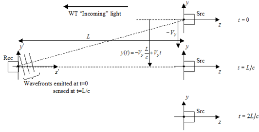
From this sketch, we conclude that tilt of the received wavefront at t=L/c is ytilt' = -Vy/c (the minus sign is consistent with the WaveTrain tilt sign conventions). If the corresponding WaveTrain system is constructed with PointSource, AtmoPath, and SimpleFieldSensor or Camera blocks, the user can confirm that this is the tilt answer reported by WaveTrain. In fact, the reasoning related to the delay time from the point of view of the sensor that led to the above sketch and conclusion is exactly what WaveTrain does internally.
Now the paradox arises as follows. Let us consider the situation in the rest frame of the source. The following sketch shows the receiver position at several instants. From this point of view, the
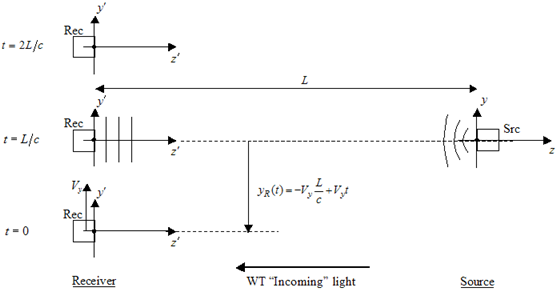
wavefronts anywhere along the z axis are perpendicular to z, so at the instant t=L/c it appears that the receiver should report ytilt = 0. This clearly contradicts the result inferred from the first approach. In an auxiliary document, we discuss this paradox at greater length, from several other points of view, and we argue that the first result (the WaveTrain result) is the correct one.
Transverse and longitudinal motion
All the commentary in this section applied to transverse motion. Issues relating to longitudinal motion are of a different character, and are discussed in a separate section.
In order to work confidently with offsets, slews and other tilt-related modules, the user should have a basic understanding of how overall tilt is internally represented in WaveTrain. Some WaveTrain modules that add tilts to a wavefront offer the user a choice of methods for representing the tilt, while other modules offer no choice, using one method only. Consider the basic Tilt module, whose i/o and parameters are shown below left.
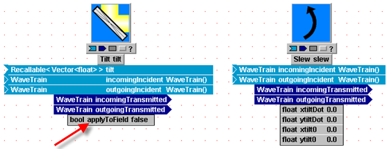
Notice the boolean (type "bool") parameter named "applyToField", which can be assigned the values "true" or "false". This offers the user a choice in how to internally represent the tilt angle that Tilt applies to the passing optical wave. If "applyToField" is set to "true", then the module will multiply the incident complex field by a phasor of the form exp[ ± i(2p/l)(Dqx x + Dqy y) ]. If "applyToField" is set to "false", then Tilt will not apply the tilt phasor, but rather will add the present tilt increment to the so-called "tilt register" for the wave in question. Unless the user's application explicitly requires otherwise, the normal setting for "applyToField" should be "false" (note this is the default setting when the module is initially added to a system): it is almost always preferable to carry overall tilt information separately from the remaining complex field array.
The difficulty that arises when "applyToField" is
"true", is that modest tilts can cause impractical sampling requirements for the
numerical propagation mesh. In a general WaveTrain diffractive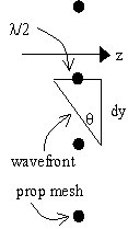 propagation module, the incident complex field array (part of the "wavetrain")
is input to a Fresnel propagation operator.
Suppose now that we wanted to explicitly apply a tilt of 100
mrad to the phase of a plane wave of wavelength 1
mm, prior to applying the propagation operator.
As shown in the sketch at right, to sample the initial tilted wavefront with
even marginal adequacy would require a mesh spacing as small or smaller than dy
= (l/2)/q
= 5 mm. This spacing may be considerably denser than required by the
other sampling constraints; furthermore, tilt angles of interest for
WaveTrain problems can easily exceed this 100 mrad
example. To avoid potentially severe sampling difficulties of this type,
WaveTrain exploits a known mathematical property of the Fresnel propagation
operation. If one applies the Fresnel propagator (along z) to a wavefront
with a specified tilt factor, the resulting complex field is exactly equal to
that obtained by propagating the tilt-removed field, shifting that result
transversely, and finally applying a tilt phasor. The latter method is
what WaveTrain uses when "applyToField" = "false" in
Tilt
and similar modules.
propagation module, the incident complex field array (part of the "wavetrain")
is input to a Fresnel propagation operator.
Suppose now that we wanted to explicitly apply a tilt of 100
mrad to the phase of a plane wave of wavelength 1
mm, prior to applying the propagation operator.
As shown in the sketch at right, to sample the initial tilted wavefront with
even marginal adequacy would require a mesh spacing as small or smaller than dy
= (l/2)/q
= 5 mm. This spacing may be considerably denser than required by the
other sampling constraints; furthermore, tilt angles of interest for
WaveTrain problems can easily exceed this 100 mrad
example. To avoid potentially severe sampling difficulties of this type,
WaveTrain exploits a known mathematical property of the Fresnel propagation
operation. If one applies the Fresnel propagator (along z) to a wavefront
with a specified tilt factor, the resulting complex field is exactly equal to
that obtained by propagating the tilt-removed field, shifting that result
transversely, and finally applying a tilt phasor. The latter method is
what WaveTrain uses when "applyToField" = "false" in
Tilt
and similar modules.
By way of contrast to Tilt, there are some closely related modules where the user is given no choice regarding the internal tilt representation. For example, the Slew module, which is illustrated on the right side of the previous diagram, is at the WaveTrain code level simply a time-varying Tilt. However, from the i/o and parameter lists, we see that Slew provides no "applyToField" option: WaveTrain automatically uses the concept "applyToField" = "false" in Slew. The following section further discusses the connection between tilt representation and the required size of the numerical propagation mesh.
Transverse displacement and size of propagation mesh
An important feature of WaveTrain is that the required size of the optical propagation mesh is, in one important aspect, decoupled from the transverse displacement or motion of sources and sensors. This feature is closely connected with WaveTrain's methods of modeling overall wavefront tilt. Before continuing with the present section, the reader should quickly review the previous section on tilt modeling, whose essentials form the background for the present section.
Consider again one of the WaveTrain
systems used previously to illustrate transverse motion and slew.
Suppose that:
(a) the transmitter-receiver z-separation is 100 km, and the receiver
velocity relative to the transmitter is vRy = +100m/s;
(b) the aperture radii of both the Gaussian laser and the receiver
telescope are 0.5 m;
(c) at t = 0, the receiver and transmitter local origins have zero
transverse offset (x0 = 0 = y0 in both TransverseVelocity modules);
(d) we wish to simulate the receiver signals until t = 0.1s .
At the end of this time interval, the target subsystem center will have a
y-offset of 10 m and 100 mrad
relative to the source center. In accordance with WaveTrain's
modeling of overall wavefront tilt, the transmitter-end
Slew module does not multiply
the exiting complex field by a tilt phasor. Therefore, it is not
necessary for the optical propagation mesh to sample the 100
mrad initial tilt or to contain the 10-m final offset
between source and sensor. It is only necessary for the propagation mesh
to satisfy the sampling requirements of the zero-offset geometry. The
zero-offset
mesh equirements are influenced by the transmitter and receiver aperture
diameters, the propagation distance, the wavelength, the integrated turbulence
strength, and the spatial spectrum of the initial complex field, but not
by the motion-induced offsets in the system. The time-varying offsets are
all handled internally by appropriate transverse shifts, and by application of
tilt phasors just prior to sensing, if the sensor type requires it.
Notice in the preceding sentences that we said the propagation mesh requirements are influenced by the spatial spectrum of the initial complex field. In particular, if for some reason the initial complex field contains a large overall tilt, then the mesh must be dense and large enough to be able to adequately sample this field for input to the propagator. But, the point is that WaveTrain's method of handling motion offsets and slew is designed to avoid the impractically large propagation mesh dimensions that would be needed if the associated tilt factors were always represented in the pre-propagation complex field.
CAUTION: WaveTrain's "applyToField"="false" method cannot by itself solve all tilt-related sampling problems. We stated above that the tilt carried in the so-called "tilt register" is finally put into the complex field just before sensing occurs. Now if the sensor is of a type that is sensitive to the incident phase in the sensor pupil (e.g., SimpleFieldSensor or Camera), then of course inadequate sampling of that phase will produce incorrect phase results. However, this problem is usually easy to circumvent, because a pre-sensor Slew can be used to orient the sensor so that the pupil plane is more or less parallel to the incident tilt. This issue was already discussed in a somewhat different form in one sub-section of the transverse-motion and slew introduction.
Transverse displacement and size of phase screens
Atmospheric turbulence models and the specification of turbulence phase-screen strengths and positions is discussed in another section. However, the desired size of the phase screens is more closely related to transverse motion, so we discuss that subject now.
The specification of the turbulence phase screen mesh parameters (dimension and spacing) is a separate step from, though logically related to, the propagation mesh specification. Desired screen mesh parameters are linked to the propagation mesh as well as to the transverse displacement of transmitter, receiver and air mass during the simulation time span. The screen mesh parameters are specified via parameters in one of the propagator modules such as AtmoPath or GeneralAtmosphere. These two modules are shown below, with their i/o and parameter lists pulled down.
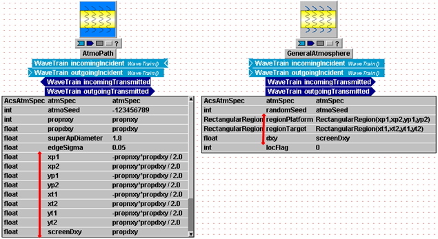
The concepts by which the screen meshes are specified in
the various propagator modules are identical, but the parameter name notation
and grouping differs slightly from one module to the next. Once the user
understands the concepts, the naming variations should not cause any confusion.
We will explain the key ideas in terms of the
AtmoPath nomenclature. The
relevant parameters in AtmoPath
(see above figure) are the two groups {xp1, xp2, yp1, yp2} and {xt1, xt2, yt1,
yt2}, plus the parameter screenDxy. The index numbers "1" and "2" should
be understood as "min" and "max":  thus, the coordinates {xp1, xp2, yp1, yp2} define a rectangular region at the
platform (p) side of AtmoPath,
while the coordinates {xt1, xt2, yt1, yt2} define a rectangular region at the
target (t) side of
AtmoPath. The sketch at
right illustrates the y dimension. (Note that
the parameter values entered in the above AtmoPath diagram (third column
in the parameter list) are merely the default values that are presented when one
initially pastes AtmoPath into a user system.)
thus, the coordinates {xp1, xp2, yp1, yp2} define a rectangular region at the
platform (p) side of AtmoPath,
while the coordinates {xt1, xt2, yt1, yt2} define a rectangular region at the
target (t) side of
AtmoPath. The sketch at
right illustrates the y dimension. (Note that
the parameter values entered in the above AtmoPath diagram (third column
in the parameter list) are merely the default values that are presented when one
initially pastes AtmoPath into a user system.)
Once the user specifies values for the p-side and t-side rectangular regions, WaveTrain conceptually connects the endpoints by straight lines (dashed lines in the sketch), forming in two dimensions a rectangular frustrum. Finally, at the designated z coordinates of the phase screens (zsk in the sketch), WaveTrain creates phase screens that span the interior of the frustrum (as indicated one-dimensionally in the sketch). The rectangular frustrum algorithm is a general method for more or less optimizing the required sizes of the successive phase screens. In sum, by specifying rectangular x-y regions at the platform and target ends of the propagator module, the user implicitly specifies the size of all phase screens that will be used in that propagator module.
How large should the p-side and t-side rectangular regions be? The rectangles at the two ends must be at least as large as the propagation meshes used, and frequently should be larger, for two reasons. First, as the transverse positions of platform, target, and air mass evolve (assuming there is motion), the optical beams sample different portions of the phase screens. Ideally, the size of the p-side and t-side rectangular regions would be chosen so that at a given screen z the screen spans the entire width swept by the beam during the simulation. In practice this may not be feasible for long simulation times, so WaveTrain has the following provision. If the user-specified size of a screen is insufficient to span the area required by transverse motion, then WaveTrain automatically wraps the screen. Equivalently stated, whatever the user-specified size of the screen, WaveTrain will treat that screen as a periodic function whose period is the screen "size" specified by the user. As a result, any optical beam will always have some phase perturbation to sample, although that perturbation may repeat itself in time at a particular screen location. After we illustrate screen setup with a numerical example, we will discuss further how to avoid overall periodicity of the propagation results when we specify undersized rectangular regions.
There is also a second reason for making screen sizes bigger than the propagation mesh, which has nothing to do with motion. The issue here is a defect of the conditioned-white-noise method of generating 2D random functions. We discuss this second issue a bit more in a later section on screen details.
Numerical example of screen width specification based on motion
Let us consider a numerical example to illustrate the screen mesh specification. Consider again one of the WaveTrain systems used previously to illustrate transverse motion and slew. We repeat the system diagram here:
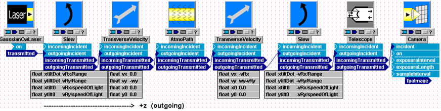
Suppose that:
(a) The transmitter-receiver z-separation is 100 km
(b) The platform velocity relative to earth is (0, 0)
(c) The receiver velocity relative to earth is (vRx, vRy) = (-20, +100)m/s
(d) The true-wind velocity relative to earth is (0, wy) = (0, +10 m/s)
(e) At t = 0, the receiver and transmitter local origins have zero
transverse offset (x0 = 0 = y0 in both TransverseVelocity modules)
(f) We wish to simulate the receiver signals until t = 0.1s (= Tsim)
(g) The propagation mesh parameters propnxy (dimension) and propdxy
(spacing) have been specified as discussed elsewhere,
and for brevity we define DXYprop
= propnxy * propdxy. (The x and y specifications of the propagation mesh
are not required to be equal, but that is a common case). Suppose that
DXYprop = 4 m has been
specified.
We discussed in a previous
section how the motion specifications (b)-(e) translate into the (vx,vy) and
(x0,y0) value specifications that have been entered in the third columns of the
two TransverseVelocity
blocks. We are now in the process of determining the turbulence screen
parameter values to be entered in
AtmoPath. The key facts are:
(1) At the platform (z=0), the total displacement of the source modules
relative to the atmosphere during the simulation time is (DXp,
DYp) = (0, -wy*Tsim) = (0,
-1.0) m.
(2) At the target end, the total displacement of the atmosphere relative
to the target modules during the simulation time is (DXt,
DYt) = (-vRx*Tsim,
[wy-vRy]*Tsim) = (2.0, -9.0) m.
(3) The propagation mesh spans (DXYprop,
DXYprop) = (4.0, 4.0) m.
As explained elsewhere, because of WaveTrain's motion/wavefront-tilt procedures,
we can think of the propagation mesh as
having zero offset at all times despite the transverse motions.
Combining the maximum motion offsets with the size of the
propagation mesh, i.e, the facts (1)-(3), we can fix phase screen sizes
(regardless of their z locations) by specifying the following rectangular
regions in AtmoPath:
(A) (xp1, xp2) = (-DXYprop/2,
DXYprop/2)
= (-2.0, 2.0) m
(yp1, yp2) = (-DXYprop/2,
DXYprop/2 + | wy*Tsim |)
= (-2.0, 3.0) m
(xt1, xt2) =
(-DXYprop/2,
DXYprop/2 + | vRx*Tsim |)
= (-2.0, 4.0) m
(yt1, yt2) =
(-DXYprop/2,
DXYprop/2 + | wy-vRy |*Tsim)
= (-2.0, 11.0) m.
For each pair of coordinates, we have added the absolute value of the
relevant motion displacement to the upper bound of the zero-offset propagation
mesh. Adding the magnitudes in this way is not the only viable approach,
but it has one significant advantage. First, note that the screen
periodicity discussed earlier means that (xp1, xp2) and the other pairs can be
extended in either direction: it is not obligatory to extend the
rectangular regions in the actual direction of motion. The principal
advantage of using the absolute value method illustrated in (A) is that the
algebraic combinations remain valid if one later changes the signs of the
various velocities when executing parameter studies of the system behavior.
The alternative method, which might initially seem more
straighforward, is illustrated by the following specification:
(B) (yp1, yp2) = (-DXYprop/2
- wy*Tsim,
DXYprop/2)
If wy = +10 m/s, as in the original numerical specification, then the yp1
assignment in (B) explicitly accounts for the fact that a screen located at the
platform would move towards +y by the amount DY
= wy*Tsim, relative to the platform. But now a potential problem arises:
suppose we defined yp1 algebraically as in (B), elevating the wy variable up to
the runset where a numerical value is assigned. Suppose further that at
some later time we are exploring parameter variations and we decide to assign a
negative value to wy. Inspection of the (B) format shows that an error
occurs unless we move the wy*Tsim contribution from the yp1 to the yp2 term.
Similarly, in the term (wy-vRy) a net sign change can occur depending simply on
whether wy is less or greater than vRy. As a general principle, it is
inconvenient and error-prone to set up the system and runset so that changing
the numerical value of a runset parameter requires us to make some compensating
setting change lower down in the system hierarchy. For some system
properties it may become too involved to maintain complete generality in this
respect, but for the screen specifications the absolute value method (A)
provides an easy solution.
In the specifications (A), we concluded with numerical values to give a sense of typical numbers. However, we would generally want to enter the algebraic setting expressions in AtmoPath, and to elevate variables like wy, vRy, etc. to the runset level: that makes it easy to perform parameter variations by just changing a few numbers in the runset. Detailed syntax rules and elevating procedures are discussed in other chapters; to conclude the present discussion we just point out one pertinent detail, namely that |x| must be entered in WaveTrain setting expressions as fabs(x).
Actual screen dimensions, computation time and memory requirements:
Thus far, the present section has concentrated on specifying the physical span of the turbulence phase screens. The final parameter required to specify the discrete screens is the mesh spacing, which in AtmoPath is called screenDxy. Typically, we set screenDxy equal to the propagation mesh spacing designated in some previous expressions as propdxy. Strict equality of screenDxy and propdxy is not obligatory, but is usually a reasonable choice.
Once the user has specified the spans (xp2 - xp1), ..., and the screenDxy, then the screen meshes are fully specified as far as the user is concerned. However, WaveTrain makes some further internal adjustments. At present, WaveTrain generates phase screens by starting with an uncorrelated random process in the frequency domain, spectrally conditioning that power spectrum, and then inverse transforming to obtain the space-domain screen realization. Since the Fast Fourier Transform (FFT) algorithm is used, WaveTrain adjusts the ratio (xp2 - xp1)/screenDxy upward to the nearest integer having a "nice" factorization for evaluating the FFT. Thus the screen dimension will actually be slightly bigger than implied by the precise user specifications.
Screens are only generated once per atmospheric realization, so that even very large screens may have small impact on simulation execution time. Propagation and motion evolution requires Fresnel propagation from source to first screen, then from screen to screen, then finally from last screen to sensor, for each time step of the simulation, but all with a single pre-computed set of screens (a single atmospheric realization). Therefore, even if the screens are much larger than the propagation mesh, it is often the case that execution time is dominated by the propagation calculations, and is only slightly affected by the initial generation of the screens. Of course the screens are used at each propagation step, but after the screens are generated by using the spectral conditioning method then each screen application during propagation is only a simple array multiplication.
On the other hand, required memory is strongly affected by the specified screen size. We cannot give specific limits on screen dimensions for various computer configurations, but we can give a few examples of dimensions that have been used with no ill effects. In the numerical example of screen specification given several paragraphs ago (at the (A) marker), the target-end rectangular region spanned 6x13 m in the XxY dimensions. Supposing that screenDxy=2 cm, that would imply (prior to the WaveTrain adjustment) a screen dimension at the target end of 300 x 650 points. This is a modest requirement in terms of modern personal computers. If we increased Tsim from 0.1s to 1.0 s, then the 6x13 m becomes 24x94 m, or a screen dimension of 1200x4700 points. This is still doable on a modern PC, but may be approaching the danger zone depending on the user's PC configuration.
Avoiding overall periodicity by various means
We noted above that WaveTrain's phase screens effectively scroll periodically if relative motion requires an optical propagation operation to sample a phase screen beyond its nominal edge. If all the phase screens repeated with the same frequency, then the optical results at a sensor would repeat exaclty with that frequency, making runs longer than that period useless. If there is a need to accumulate statistics over longer periods, several approaches can be considered.
The brute-force approach is to make the screens longer in the direction of motion, but as discussed above this has practical computer limits.
A simple approach would be to do repeated runs with different random number seeds for the screen set. The repeated runs cannot be joined end to end in post-processing because discontinuous jumps in results would occur at the joints. However, the method is perfectly satisfactory for accumulating certain types of statistics.
Another possibility is to note that overall periodicity can be mitigated significantly if the screens have different lengths or different transverse speeds. In that case, even though each screen is repeating periodically, the combined turbulence effect would only repeat over a much longer period, namely the least common multiple of the individual periods. Although some violation of nature is involved here, for most statistical purposes the approximation is probably quite good.
Longitudinal (z) displacement and motion
WaveTrain has no facility for representing longitudinal motion comparable to the modules provided for representing transverse motion. In most WaveTrain applications of interest, the longitudinal component of motion does not produce any noticeable change to the measured quantities of interest: it is only the transverse components of the physical velocities that generate the turbulence-related time dependences of modeling interest. The longitudinal components are insignificant because of the combination of the relatively large propagation distances involved, and the relatively short time spans over which we need to perform the wave-optics simulation. These approximations are tied to the conventional way in which the frozen turbulence approximation is applied to optical turbulence calculations.
There are several limitations to this physical model. The first limitation has nothing to do with turbulence, but arises simply because various magnification factors change if the distance changes significantly during the simulation time. A second limitation is that, as the motion progresses, phase screens nearest the target or platform should drop out of the problem when that part of the air mass is no longer between the platform and target. Modeling such changes may become important, for example, in simulating a long-enough engagement against a nearby missile moving more or less directly at the platform. At present, if such effects are important in a WaveTrain simulation, the user must break up the problem into time segments such that the z-range can be treated as approximately constant during each segment.
Despite the absence of longitudinal-motion library modules, there is a significant aspect of longitudinal motion that can be modeled in WaveTrain. Depending on the range and time scales involved, the principal effect of longitudinal motion may be a Doppler shift. A physical example is the problem of remote Doppler vibrometry through a turbulent medium. In problems of this type, we can model the longitudinal motion in terms of temporally-varying phase shifts. This produces effects such as walking fringes, for example, and WaveTrain does contain modules that can generate these effects. An auxiliary document contains a detailed explanation of how to model such effects in WaveTrain. The auxiliary document also discusses in general the extent to which the interference of polychromatic fields can be modeled in WaveTrain.
The numerical implementation of wave-optical (i.e.,
diffractive) propagation is a large subject. Here in this User Guide, our
intent is to specify a few key formulas that outline the concepts and numerical
algorithms used by WaveTrain to propagate optical fields from one transverse
plane to another. The discussion here will not fully justify the reasons
for choosing one numerical procedure over another, nor will it fully explore the
details of the numerical algorthms used in WaveTrain. What we hope to
accomplish in this User Guide discussion is:
(1) To give the user who has some acquaintance with scalar diffraction
theory (and its Fourier-transform representations) a clear general idea of which
propagator formulas are used in core WaveTrain propagation modules
(2) To use the knowledge in item (1) to make the user comfortable with the
terminology and logic involved in setting mesh and distance parameters in core
WaveTrain propagation modules
(3) To give the user an overview of WaveTrain's ability to model
non-monochromatic versus monochromatic propagation.
One can group WaveTrain diffractive-propagation modules
into two categories:
(1) Fresnel-propagation modules that propagate an optical field from one
transverse plane through some arbitrary distance to another transverse plane
(2) Fraunhofer-propagation modules that take an incident optical field,
and then propagate to (or perhaps near) the focal plane of an assumed lens.
The most commonly-used modules that set up or perform Fresnel propagation are PropagationController, AtmoPath, and VacuumProp. The PropagationController does not actually carry out any propagations, but it can be used for setting key propagation parameters. AtmoPath is a complicated component that contains phase screen action as well as multiple, sequential Fresnel propagation action. VacuumProp is more basic in the sense that it carries out one propagation over a single specified distance.
The most commonly-used module of the Fraunhofer group is Camera. Another important Fraunhofer-propagation module is HartmannWfsDft, which models a Shack-Hartmann (or plain Hartmann) wavefront sensor.
Mathematical representation of the optical field
The core WaveTrain propagation procedures apply directly to scalar, monochromatic, paraxial optical fields. The general mathematical representation of such a field is
(Eq. 1) Y(x,y,z,t) = U(x,y,z)· exp[ i (kz - wt) ]
where k = 2p/l, w = ck, z is the nominal propagation direction, U is complex, and U(...,z) is slowly varying compared to kz. Any WaveTrain propagator module operates on an input complex field given in some plane z1, of the form
(Eq. 2) U1(x,y) = A1(x,y) · exp[ i·f1(x,y) ]
The output of the propagator module is the corresponding complex field, U2(x,y), in the specified final plane of constant z2. Of course, WaveTrain actually works only with samples of U1,2 on discrete transverse meshes (x1i,y1j), (x2i,y2j). The terminology "nominal propagation direction" implies that small tilts or beam spreading around the z direction are supported by the WaveTrain propagation machinery: i.e., WaveTrain makes paraxial approximations. WaveTrain also contains special provisions for modeling the paraxial region of point-source and rough-reflector optical fields, which would normally spread far outside the paraxial regime.
The optical-frequency factor in (Eq. 1), exp(-iwt), is completely ignored in the WaveTrain propagation modules. However, in the U1,2(x,y) expressions manipulated by WaveTrain, there is an additional, slowly-varying time dependence that is not contained in the fundamental representation of (Eq. 1). That degree of freedom is that the U1,2(x,y) fields can evolve temporally (but very slowly compared to
wt), in accordance with transverse motion of turbulence screens, sources and sensors, and in accordance with the time-of-flight delay (z2-z1)/c. The propagator operation that creates U2(x,y) from U1(x,y) is itself unaware of any time tags, but transverse motions that occurs between sensor exposures, or during time of flight lags between phase screens, will cause a propagated output field to interact with a different portion of a receiver aperture, a phase screen, or whatever is acting at the z2 end. Likewise, the time at which a sensor receives a certain wavefront lags by the appropriate time-of-flight the time at which this wavefront was initiated at some source. Such lags can be vital to the correct modeling of wavefront dynamic control systems, and a consistent accounting of such lags is a strength of the internal WaveTrain machinery.The field U1's monochromatic wavelength, l, is specified and used by the propagator formulas to determine diffractive effects. However, WaveTrain propagators always ignore the absolute overall phase factor, exp[ ik·(z2-z1)] = exp[ ik
Dz ]. In the vast majority of WaveTrain applications, this overall phase is immaterial. If a user's application really requires a specific absolute fringe position at a specific time, an extra WaveTrain component can be inserted in the system model to enforce that.In the initial paragraph, we stated that WaveTrain's propagators work, strictly speaking, with monochromatic fields. WaveTrain can treat the propagation of multiple discrete wavelengths and, to various levels of approximation, the propagation of beams whose optical spectrum has finite (continuous) width. The subsection on "Non-zero optical bandwidth", located later in the present "Theoretical background" section, outlines some general concepts and procedures that allow WaveTrain to be applied to fields that are not strictly monochromatic.
The degree to which finite optical bandwidth is supported, as well as the limitations of the scalar, paraxial approximations are complex subjects which are not fully explored in this User Guide. The WaveTrain limitations are due to analytical approximations in the fundamental formulas, as well as to practical sampling limitations in the numerical discrete spatial meshes and time steps. By scanning the contents of the User Guide, readers will find other sections that also contain information pertinent to these issues. But, to a large extent, WaveTrain users must take the description of the wave propagation and sensing methods given in this Guide, and then apply their own physics understanding to determine whether a WaveTrain model can accurately represent a problem of interest. Sometimes, a bit of specially-directed numerical experimentation will be helpful. Also, consultation with MZA is available for general help on such questions.
Excellent general references for the underlying theory of
scalar, paraxial, diffractive propagation are
(1) Goodman, Introduction to Fourier Optics, McGraw-Hill, 1968
(2) Saleh and Teich, Fundamentals of Photonics, Wiley, 1991.
Propagation in the Fresnel regime between planes z1 and z2 can be expressed in the space domain or the spatial-frequency domain. WaveTrain's core numerical propagator works in the spatial-frequency domain. This fundamental propagator formula, to be found in standard texts, is
(Eq. 3):
The vector
denotes the x and y components of spatial frequency (cycles/m),
and the overbar notation is used as a shorthand for the (-i) Fourier
transform. In words, this propagator acts in three stages: (i)
compute the Fourier transform of the space-domain complex field at z1,
(ii) multiply by a quadratic-phase distance-propagation factor in the frequency
domain, (iii) compute the inverse Fourier transform to obtain the
space-domain complex field at z2.
For numerical propagation, WaveTrain uses a modification of this formula wherein a "reference curvature" phasor is factored off from U. That is, we define the related quantity V, where
(Eq. 4)
and where zR is the "reference focus" distance (directed). (zR may be set to infinity, in which case V=U). Substituting (Eq. 4) into (Eq. 3) and regrouping terms yields the propagator formula
(Eq. 5)
where the "magnification" factor M = (zR - Dz) / zR = 1 - (Dz / zR). M may be less than or greater than 1, depending on the sign of zR. When M=1, (Eq. 5) reduces to the original (Eq. 3). The following figure shows why M is called the "magnification".

The motivation for introducing the reference curvature, or equivalently M, is that in some applications the physical beam cross-section converges or diverges greatly. In such cases, we desire the NxN points of the discrete propagation mesh to span a much smaller or much larger transverse distance at z2 than at z1. If the propagator Eq. (5), with a specified M factor, is evaluated using the Discrete Fourier Transform (DFT), then the transverse space mesh is automatically compressed or stretched by the factor M. This is a natural consequence of the two DFTs in Eq (5), as the following argument shows. The first DFT, i.e., the computation of V1(bar), yields Fourier transform values on a frequency mesh of spacing
Du = 1/(NDx1), and similarly for y. Next, the quadratic phase factor containing n2 is simply evaluated on that frequency mesh. Then, when another DFT is used to compute the final inverse transform, we obtain field values on the space mesh (Dx2/M) = 1/(NDu) = Dx1 , or Dx2 = MDx1.The logic in the above paragraph is predicated on the space-frequency mesh constraints of the Discrete Fourier Transform. The specific computational algorithm used to evaluate DFTs in WaveTrain is the so-called Fast Fourier Transform (FFT).
Specifying the reference focus in WaveTrain components
The reference curvature factor, or equivalently the mesh magnification factor M, is specified in WaveTrain propagator components via the reference focus distance (directed) zR. For example, the key PropagationController or AtmoPath components contain parameters named xReferenceFocus and yReferenceFocus. Typically, one would set the two to the same value, but WaveTrain allows separate Mx and My specifications in case of highly asymmetric problems. To use M=1, x{y}ReferenceFocus should be set to 0.0. The value 0.0 is a flag here that is interpreted as infinity focus, and this is always the default value in the WaveTrain propagator components.
We emphasize that many (perhaps most) WaveTrain applications can use the M=1 specification. Particularly if we propagate a beam in the atmosphere for a few hundred meters or kilometers or more (depending on the aperture size), there is no possibility of a greatly reduced focal spot. In many such cases, there is no need to deviate from an M=1 mesh. Additionally, there are other factors besides diffraction that need to be considered to determine the mesh sample spacing. For example, suppose we have a beam that is diverging, but is propagating through significant turbulence along the whole path. In that case, we probably want to keep the mesh spacing constant as we propagate from turbulence screen to screen. .
WaveTrain nomenclature: "planar reference wave" and "spherical
reference wave":
The M=1 case is often referred to in WaveTrain documentation as the
"planar reference wave" case, or sometimes as the "plane-wave" propagator case.
The latter name may be misleading, in the sense that there is no implication
that the full wavefront is planar anywhere.
Any M
Note that zR could be the actual best-fit curvature radius of U1, but that match is not necessary. The choice of zR is arbitrary, and can be used to set the grid magnification M as desired.
Components like Camera or HartmannWfsDft propagate an incident complex field U1 to the focal plane of an assumed lens of focal length f. The propagation formula used in these cases is the space-domain Fraunhofer-regime formula
(Eq. 6):
As in the Fresnel case, the exp(ikf) factor is neglected. The DFT (implemented with the FFT) is again used to numerically evaluate the Fourier transform in (Eq. 6); the implications for the space mesh on which U2 appears are different than for the Fresnel propagator discussed previously. These mesh consequences and choices are discussed in the User Guide sections devoted to the camera sensor and the wavefront sensor.
Overall tilt and optical propagation
In a previous User Guide section, we discussed how overall tilts are typically modeled in WaveTrain. We explained there that large tilts introduced by tilt modules and sensor-source relative displacements are generally tracked separately by WaveTrain, and not incorporated into the propagating U(x,y) as a tilt phasor factor. This is done to avoid overly stressing sampling requirements in the numerical propagators. At a sensor, the separately-tracked tilt is finally inserted into the field or irradiance map by using the shift-invariance properties of the propagator.
Multi-frequency propagation and non-zero optical bandwidth
First, let us emphasize that any number of monochromatic beams of arbitrarily separated wavelengths can be propagated in a single WaveTrain system and run. To give a physical example of interest in adaptive optics: it is a simple matter (in terms of the multi-wavelength specifications) to study the performance degradation when a different wavelength is used for wavefront sensing than is used for the science imaging or laser beam projection. When propagating beams of different wavelengths, key questions are whether these beams interact at all, and if so, whether they add coherently or incoherently at a sensor. The answer depends (i) on whether a sensor is allowed to see multiple beams, and (ii) on the WaveTrain rules built into the sensor module.
WaveTrain has been validly used for many situations which
go well beyond the strictly monochromatic regime. Depending on the
problem, different approaches and justifications are used. Without going
into details, we list a few concepts and procedures applicable to
non-monochromatic cases:
(1) Accept a completely monochromatic model, realizing that many
turbulence and diffraction effects do not change that rapidly with wavelength.
This is completely satisfactory for many narrow-band propagation problems.
(2) Model a finite-bandwidth beam as a superposition of
discrete-wavelength, closely-spaced, but incoherent monochromatic beams.
(3) Explicitly introduce a slowly-varying envelope function to rigorously
model either a finite optical bandwidth, or the dynamic interference between
closely-spaced discrete frequencies.
(4) Model an extended incoherent source plane in terms of many
spatially-separated point sources, whose intensity maps will be added
incoherently at a sensor.
(5) Combine a monochromatic WaveTrain source with specialized WaveTrain
rough-reflector models. Several reflector models in WaveTrain contain
features that mock up a finite bandwidth of the illuminating source, to various
levels of fidelity. (I.e., some rough-reflector models in WaveTrain act as
specialized "secondary" sources).
Choosing mesh settings for optical propagation
The previous User Guide section on optical propagators gave background information on the propagation formulas used in WaveTrain. In the present section we complete that discussion by giving guidelines for specifying the discrete propagation mesh parameters that must actually be entered in WaveTrain model setup. Most prominently, these are the spacing of the mesh and the span (or dimension) of the mesh.
The size and spacing of the propagation mesh must be chosen very carefully; the spacing must be neither too large nor too small, and the mesh size must be large enough to capture the effects of interest, but making it too large can slow the simulation drastically. To a first approximation the execution time of most WaveTrain models varies roughly as the square of the propagation mesh dimension, so using 512x512 meshes takes roughly four times as long as using 256x 256 meshes.
To choose the mesh size and spacing correctly, there are a number of factors that must be taken into account, including
**********
UPDATE: An updated, revised and generalized discussion of the mesh
selection guidelines that appear below is available in a
separate document.
Also, the guidelines in that document have been incorporated in the
auxiliary PropConfig tool that is part of the
WaveTrain 2010A release. Users who run the PropConfig tool as part of
WaveTrain model building will find a PropConfig tab where suggested mesh
specifications are computed, based on the user-supplied propagation scenario and
the analysis in the just-referenced document.
**********
There are two main requirements: First, the mesh spacing must be small enough to adequately sample the variations in phase of both the wavefront and the quadratic phase factors applied by the Fourier optics propagator. To be specific, the phase difference between adjacent mesh points should never exceed half the wavelength. Second, the mesh extent must be large enough to capture all the propagated light, otherwise, as a consequence of the periodicity of Fourier transform, the light leaving one side of the mesh will reappear on the other side of the mesh; this effect is known as "wraparound". The two requirements are interrelated, because(1) the mesh spacing governs the maximum spatial frequency (and hence the maximum propagation angle) which can be represented on the mesh, (2) the sampling requirement for the quadratic phase factor increases linearly with the size of the region of interest, and (3) the mesh extent at each end should generally be at least twice as big as the region of interest at that end. The propagation distance and the choice of reference wave both affect the magnitude of the quadratic phase factors, and with a spherical reference wave the mesh extent and mesh spacing vary linearly along the path. Turbulence introduces additional phase perturbations - see How turbulence is modeled - and these enter into the phase sampling requirement. In some cases it is possible to mitigate wraparound effects, and thereby relax the requirement on mesh extent to some degree using spatial filters and/or absorbing boundaries - see How to use spatial filters and absorbing boundaries. The physical dimensions and configuration of the sensors used can generally be ignored, because WaveTrain will automatically interpolate the mesh at the entrance pupil as needed; however if you wish to avoid interpolation error you can choose the mesh spacing and offset accordingly. The FFT package governs what mesh dimensions are permitted, and WaveTrain can be used with several different FFT packages; some allow only powers of two, while others allow any integer which factors into powers of small primes, e.g. 2, 3, 5, and with at least on factor of two. For the Windows implementation of WaveTrain the FFT package used for optical propagation (provided by Intel) requires that the mesh dimension be a factor of two. A separate FFT package, more general but less efficient, is used for generating phase screens, but that those dimensions are set automatically anyway. Whatever the mesh dimension is, for a mesh of dimensioned n x n, by default the (n/2+1, n/2+1) point is assumed to fall on the optical axis.
We've spoken of the "regions of interest" at either end of the propagation path without precisely defining what we meant. For an optical system, the effective region of interest is closely related to the system aperture, but generally somewhat larger, to account for scattering effects. For example, when modeling the light incident on the aperture from a point source, we cannot model all of the light emitted by the point source, given the finite size of our meshes, so instead we model only that portion of the light which contributed to the wavefront received at the aperture. But with turbulence light will be scattered both into and out of the aperture; and with a true point source equal amounts would be scattered in and out on average. To match this in simulation we must consider a region containing the system aperture, and with enough of a margin on all sides that the light scattered out at the edges will not affect the average intensity across the aperture. For more details see modeling point sources. Similar considerations apply when modeling the light from an extended incoherent source, or a coherent reflection off an optically rough surface. At the other end of the path it is much the same, except that the physical extent of the object being imaged and/or illuminated plays the same role as the system aperture.
Consider the simplest case, where (1) we would use a planar reference wave, (2) the quadratic phase factors applied by the propagator dominate the phase sampling requirement, and (3) neither spatial filters nor absorbing boundaries are used. In this case the mesh requirements can be computed easily. Let l be the wavelength, z be the propagation distance, D the maximum extent of the regions of interest at the two ends, nx the mesh dimension, and dx the mesh spacing. For a given l and dx, the minimum and maximum propagation angle are -l/dx and l/dx, implying that light from any point on the mesh could expand to fill a region of size lz/dx after propagating a distance z. To avoid wraparound, the mesh extent should be at least twice that:
nx*dx >= 2lz/dx
This can be put in the form of an inequality for dx in terms of nx, or vice versa:
dx >= sqrt(2lz / nx)
nx >= 2lz / dx2
If D corresponds to the diameter of the aperture of an imaging system, l/D is the classical resolution limit for the system. Generally, dx should be no larger than lz/D, the projection of that angle over the propagation distance. Putting that value in for dx in the inequality for nx gives us the minimum permissible nx, given our assumptions.
nxmin = 2lz / (lz / D)2 = 2D2 / (lz)
For example, if l=10-6m, z=50km, and D=1.0m,
nxmin = 2*1.0*1.0 / (10-6*50,000) = 40
However, in order to use that nx, we must use the maximum value allowed for dx:
dxmax = lz/D = (10-6*50,000)/1.0 = 0.05m = 5cm.
Also, with those choices for nx and dx the mesh extent is just twice the aperture diameter. For many cases of interest that will not be acceptable, because a denser mesh will be required to properly sample turbulence effects, and because we must consider a region of interest larger than the aperture, as discussed previously. To decrease dx, we must increase nx, and it goes as the inverse square, so to halve dx, to 2.5cm in this case, we must quadruple nx, to 160. That would double the mesh extent, from 2.0m (40*5cm) to 4.0m (160*2.5cm), allowing us to enlarge the region of interest. For most cases involving propagation through turbulence, if we choose a mesh spacing sufficient to adequately to sample the turbulence effects, then choose nx to satisfy nx >= 2lz / dx2; that will give us more than enough room for the region of interest. Bear in mind that nx must be a valid dimension for the FFT package being used.
So the question arises, how should one pick dx, given the range, wavelength, and turbulence distribution? There is no hard and fast answer, because it depends on the degree of accuracy required, but as a general rule the maximum permissible dx will vary in proportion to the coherence length, which characterizes the spatial variation of the phase of a wavefront which has been propagated across the path of interest. For a planar reference wave we recommend that dx should be no greater than one fourth the minimum of the two plane wave coherence lengths, one computed in each direction. For a spherical reference wave we recommend that the dx at each end should be no greater than one fourth the plane wave coherence length computed in the corresponding direction. But for maximum surety, when modeling a propagation scenario different from those you've modeled previously, it is always a good idea to double-check that the dx you have picked is small enough. To do this, pick a few of the more stressing cases you plan to model, and run simulations both using the dx you hope will work, and also using a smaller dx, with a correspondingly larger nx. Compare the results - whatever results are relevant to your application - and use the differences between the corresponding runs to estimate the margin of error. As an example, below are shown the aperture plane intensity and phase obtained using three different choices of nx and dx for the same propagation scenario.

Incidentally, these results were generated using WtDemo, the system model created in the course of our step-by-step tutorial. The case we used approximates typical conditions at the Airborne Laser Advanced Concepts Testbed (ABL ACT) atop North Oscura Peak, on the White Sands Missile Range, in New Mexico.
When using a spherical reference wave the requirements pertaining to mesh extent and mesh spacing are much the same, but you now have an additional degree of freedom, the placement of the point to which the reference wave is converging to or diverging from, and that can sometimes be useful, especially when the region of interest is much larger at on end of the propagation path than it this at the other. But the sampling requirements must still be satisfied, and the mesh spacing increases in direct proportion to the mesh extent, so that will often be the limiting factor. Also, it is important to remember that since the reference wave is now curved, the phase difference between the reference wave and a wavefront with similar curvature is reduced, which tends to ease the sampling requirements, but the phase difference is increased for wavefronts that are basically flat or of the opposite curvature. It can be shown that the reference wave which minimizes the mesh dimension required to adequately sample spherical waves propagating in both directions is precisely that which projects the region of interest at one end to that at the other. Unfortunately there is no similarly simple criteria to ensure that turbulence effects are adequately sampled, but, as with planar reference waves, you can make an educated guess, based on the coherence length in each direction, then double-check.
WaveTrain supports rectangular propagation meshes - ny need not be equal to nx. Both, however, must satisfy all sampling requirements, but the requirements for the two axes may differ, because the extent of one or both regions of interest may be greater in one direction than in the other. At this time the spacing in both directions must be the same (i.e., dx = dy). Rectangular meshes may be used with either planar or spherical reference waves, the latter subject to the above caveat. It would be straightforward to add support for differing spacings in the two directions, and we could also add support for reference waves with different curvatures in x and y, both of which may be useful in modeling imaging and/or illumination of objects much longer in one direction than the other. If you think those capabilities might be important for your application, please contact us.
Once you have determined the mesh dimensions and spacing you wish to use, you need to put that information into your system model. This can be done using either of two components AtmoPath (the component usually used to model propagation through turbulence), or PropagationController, which gives you more detailed control. AtmoPath actually contains two PropagationControllers, inside it, one for each propagation direction, but most of their parameters have been hardwired, to make AtmoPath simpler to use. The reference wave is planar, the propagation mesh is square, and no spatial filtering or absorbing boundaries are used. The default modeling approaches for both point sources and speckle are used, both of which make use of the parameters superApDiameter and edgeSigma, which the user can specify. For details, see How point sources are modeled and How speckle is modeled. When AtmoPath is used, all propagations in both directions are modeled using all the same modeling parameters. Because of these simplifications, only four optical modeling parameters remain to be set:
propnxy the mesh dimension (same in x and y)
propdxy the mesh spacing (same in x and y)
superApDiameter used in modeling point sources and/or speckle
edgeSigma used in modeling point sources and/or speckle
Note: the other parameters of AtmoPath relate to modeling atmospheric turbulence, and their use is described in How turbulence is modeled.
Setting up Fresnel propagations
In the previous section on specifying propagation mesh settings, we discussed the selection of numerical values for a Fresnel propagation mesh. There are several types of WaveTrain library components that accept propagation mesh parameters and compute propagations, and these systems may be used in various combinations. The ways in which the combinations are used may be somewhat confusing to new WaveTrain users, so in the present section we illustrate the basic combinations. Subsequent sections give more details on the input and parameter specifications for the individual WaveTrain components.
The principal confusion that may arise is that some components, in particular AtmoPath and its derivatives, accept both propagation mesh and atmospheric turbulence specifications. On the other hand, in more advanced WaveTrain work, it may be desirable for users to insert separate components to specify propagation mesh as opposed to atmospheric specifications. Without further ado, the following figure illustrates several different combinations of WaveTrain library components that could be used to specify the propagation mesh and atmospheric (or vacuum) parameters.
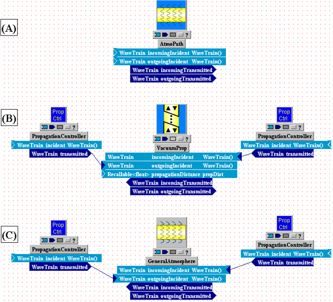
Bear in mind that, to make complete WaveTrain systems out of the above combinations, one must add source and sensor components. Now we make some general comments on each of the combinations (A-C):
(A): The single component AtmoPath can provide complete specification of both the propagation mesh parameters and the atmospheric turbulence parameters. We recommend that new WaveTrain users start with option (A). Notice that propagation in both directions ("incoming" and "outgoing") through the same specifications is supported. Note that AtmoPath subdivides the total specified propagation length into propagation segments between the turbulence phase screens.
(B): Option (A) can be used to model non-turbulent propagation ("vacuum propagation"), by setting phase screen strengths to zero. However, for clarity, users may instead wish to use the explicit VacuumProp component. But, VacuumProp takes only a propagation distance specification, not a complete propagation mesh specification. Therefore, one or two PropagationController components must be joined to the propagation module. If propagation will be only one way, then only one PropagationController is needed.
(C): Option (C) is actually very similar (but not identical) to option (A). If we descend into the AtmoPath component, we will see that AtmoPath is actually a "composite" WaveTrain system that consists of two PropagationControllers sandwiching a GeneralAtmosphere component. That is almost exactly like option (C), except that option (C) allows different propagation mesh specifications in the Controllers for the two propagation directions. This can be an important degree of freedom for some WaveTrain modeling. The GeneralAtmosphere is used to provide the turbulence phase screen specifications.
(D): This is not illustrated in the above figure. For two-way propagation, another option is to use two completely separate AtmoPath components, one for each direction.
For certain modeling situations, necessity dictates one or another of the options listed above. However, in other situations the choice is a matter of user preference.
Using the PropagationController
As an introduction to the present section, users should review the previous overview section on setting up Fresnel propagations.
PropagationController is a library subsystem that defines the Fresnel propagation mesh, in addition to several other propagation-related parameters. Every WaveTrain system should contain at least one PropagationController for outgoing waves, and at least one for incoming waves (if the respective waves are present). However, some commonly-used library systems that specify atmospheric turbulence already contain two PropagationControllers (one for each direction). The prime example is AtmoPath, which is a composite system consisting of GeneralAtmosphere and two PropagationControllers. Therefore, it may be unnecessary for the user to explicitly add PropagationControllers to the overall system. If the options provided in AtmoPath or analogous modules are sufficient for the user's purposes, then no extra controllers are required.
If a PropagationController is explicitly inserted, it can be placed anywhere along the path between the source and sensor to which it should apply. A situation that always requires explicit insertion of a PropagationController is a test system that has zero total propagation distance, and therefore contains no AtmoPath or analogous module. Such a system will usually be a test system used to investigate the behavior of a portion of a full propagation system. Multiple controllers in a system are also allowed: this is explained further in a later subsection.
Parameters of PropagationController
The picture below shows the interface of PropagationController. As we see from the single input and output, one PropagationController applies to one wavetrain (possibly containing numerous separate waves) traveling in one direction, either incoming or outgoing. We now discuss some of the parameters that must be set.
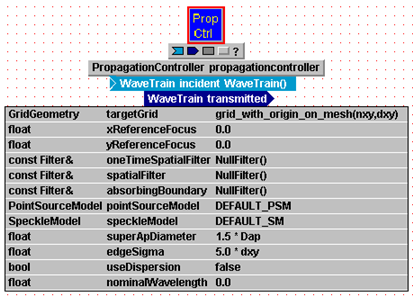
targetGrid: this parameter is set by using a WaveTrain library function that defines meshes. The user should change only the (nxy,dxy) symbols that are arguments of the function: these define the dimension and spacing of the propagation mesh. General considerations and restrictions regarding WaveTrain meshes are explained elsewhere. As usual in WaveTrain when setting parameter values, (nxy,dxy) can be replaced by numerical values right here or the symbols can be elevated (promoted) up the hierarchy. The argument syntax (nxy,dxy) may be replaced by (nx,ny,dx,dy) if the user wishes to use an asymmetric mesh. However, it is important to remember that a "long" mesh dimension is NOT required merely because there is transverse motion in the simulation (the implications of transverse motion for propagation and phase-screen meshes were discussed previously).
x{y}ReferenceFocus: these parameters allow selection of a planar or spherical reference wave for the Fresnel propagation operations. Each Focus is a directed distance in meters. Infinity focus, which is specified to the code by setting Focus=0.0, specifies a planar reference wave. The subject of reference waves is discussed in more detail in the User Guide section on optical propagators and on the selection of propagation parameters.
oneTimeSpatialFilter, spatialFilter, absorbingBoundary: these are advanced options that can be used to specify certain anti-aliasing or wrap-around measures in the Fresnel propagation FFT calculations. A few further remarks on these subjects may be found in the User Guide section on selection of propagation parameters. The NullFilter() settings shown in the above picture disables these options. User desiring further details of the available settings should contact MZA.
pointSourceModel: this setting only pertains to the operation of WaveTrain's PointSource (and derivative) source modules. The discrete numerical modeling of propagation from a point source poses special problems, and the general issues are discussed in a separate section. In brief, WaveTrain offers two methods of modeling point sources, and the desired method is selected by setting the value of the pointSourceModel parameter. For most purposes, we recommend the setting DEFAULT_PSM, as shown in the above illustration (note that PSM = Point Source Model). This selects MZA's back-propagation method of modeling the point source. If DEFAULT_PSM is used, then the associated parameters superApDiameter and edgeSigma also come into play.
superApDiameter: the diameter, in meters, of the "super-aperture" used in the back-propagation method of modeling point sources (pointSourceModel = DEFAULT_PSM). The super-aperture diameter should be somewhat larger than the diameter of the actual receiver aperture. There is no exact rule, but a factor of 1.5 is typically satisfactory.
edgeSigma: a roll-off width parameter, in meters, that modifies the "super-aperture" used in the back-propagation method of modeling point sources. A non-zero Gaussian rolloff is added to the radius of the uniform-amplitude region that is back-propagated to form the "point" source. There is no exact rule, but a typical setting would be edgeSigma = several times the propagation mesh spacing.
speckleModel: this setting only pertains to the operation of the rough-surface reflector modules, such as CoherentTarget, IncoherentReflector, and PartiallyCoherentReflector. The discrete numerical modeling of propagation from an optically-rough reflector poses special problems, and the general issues are discussed in a separate section. The setting options for speckleModel are: (a) DEFAULT_SM, (b) DELTA_CORRELATED_SM. We recommend the option DEFAULT_SM (note that SM = Speckle Model): this setting applies a super-aperture back-propagation concept to the wave propagated from a rough reflector. This means that the parameters superApDiameter and edgeSigma are also relevant to light emanating from rough reflectors, if DEFAULT_SM is selected.
useDispersion: this setting, whose allowed values are true or false, determines whether a wavelength dispersion model will be applied to the atmospheric propagation. The true setting is only applicable if at least two different wavelengths are present in the simulation system. If dispersion is applied, then nominal propagation axes will be appropriately "bent" so that beams of different colors sample slightly different portions of the atmospheric turbulence screens. The path "bending" is done relative to one of the system wavelengths, which the user specifies as the nominalWavelength
nominalWavelength: see the useDispersion parameter.
Use of multiple PropagationControllers
For reasons of convenience or user preference in building systems, it is allowed for a WaveTrain system to contain more than one PropagationController (counting the ones inside AtmoPath or analogous modules) for a given direction of propagation. If there are multiple controllers for a given direction, then the one closest (downstream) to a source overrides the settings in the others. Sometimes redundant controllers are inserted simply as a matter of user preference, but it might also happen that one wants to use different meshes or other settings to propagate different sources. The following figure gives an example:
In the model shown above, propagation from pointsource and pointsource2 is controlled by the PropagationController inside AtmoPath, but propagation from pointsource3 is controlled by the extra explicitly inserted PropagationController. All this follows from the rule "controller closest (downstream) to the source".
Using atmospheric turbulence models
WaveTrain models the optical effects of atmospheric turbulence using a standard wave optics technique, called in some references the "split-step" method. The procedure is:
(1) Divide the propagation path into a number of subintervals.
(2) For each subinterval, compute the integrated turbulence strength based on a model of the continuous turbulence strength profile.
(3) For each subinterval, generate a "phase screen" whose optical path difference map, OPD(x,y), is a statistical realization that, in the mean, corresponds to the integrated turbulence strength.
(4) Position each screen at some point within its subinterval.
(5) Using Fresnel propagator formulas, propagate the optical beam from an initial plane to the first screen, apply that phase-screen distortion, propagate the result to the second screen, apply that phase-screen distortion, and repeat until the desired final plane is reached.
The time evolution of atmospheric turbulence is assumed to obey the Taylor frozen-flow hypothesis. Thus, in addition to the above algorithm steps, we add the following:
(6) Model the time evolution of the turbulent propagation by shifting the phase screens relative to sources and sensors, by amounts consistent with the various transverse motion specifications that WaveTrain accepts.
As discussed previously, the Fresnel propagator used by WaveTrain is the spatial-frequency-domain form of the propagator. Fast Fourier Transform algorithms are used to evaluate the two transform operations required by the propagator.
Propagation time delay effects are thoroughly and consistently accounted for: all propagation time lags between screens are incorporated. The various screens receive the wavefront in precise accord with the physical propagation time lag from screen to screen. Thus, once given a full-path turbulence realization (a set of screens), all temporal and spatial correlations have correct contributions due to propagation lags between screens.
The phase distortion applied by any phase screen is expressed by
u'(x,y) = u(x,y)*ei*k*OPD(x,y).
where u(x,y) is the complex field incident on the screen, k is the wavenumber (2p / wavelength), OPD(x,y) is the screen OPD in units of meters, and u'(x,y) is the field exiting the screen.
The statistical realizations of the screens are generated in such a way as to reproduce the Kolmogorov statistics that describe locally homogeneous turbulence in the so-called inertial range. In a later subsection, we discuss the algorithm for screen generation in somewhat more detail. As a modification to the basic Kolmogorov statistics, the screen generation mechanism has options to impose an explicit inner or outer scale rolloff. The inner scale modeling uses the "Hill bump" form of the turbulence spectrum.
Any number of phase screens may be used, but in practice the maximum used is typically 10 to 20. WaveTrain allows arbitrary spacing of the screens; uniform spacing or equal-strength spacing are frequently-used special cases. Equal-strength spacing means that the full propagation distance is divided into subintervals whose nominal integrated-turbulence strengths are equal; in this case, the lengths of the subintervals are unequal, unless the continuum strength profile is completely uniform.
WaveTrain has various options for specifying the phase screen strengths. Usually the screen strengths are specified in terms of equivalent Cn2 values for the subintervals. In general, Cn2 refers to the standard refractive-index structure parameter, which in WaveTrain always has the MKS units of m-2/3.
(Background note: The Cn2 parameter is that constant which is defined by the Kolmogorov formula for the structure function of the refractive-index fluctuations:
mean{ [n(r1) - n(r1+r)]2 } = Cn2 · r2/3
where n = refractive index, and r = separation of two points in the random medium.)
Specifying effective Cn2 values for WaveTrain phase screens
For wave-optics simulation, we typically know a model profile, Cn2(z), along the propagation path. This may be uniform for near-horizontal paths, or may vary over orders of magnitude for a ground to high altitude path. Several model profiles have been developed to describe the typical variation of Cn2 with vertical altitude, h, in the earth's atmosphere. Some commonly used profiles are known by the names Hufnagel-Valley 5/7, Clear 1 Night, and SLC. (For a discussion of these and profiles in general, see the review article by Beland).
A phase screen represents the integrated Cn2 strength over the distance corresponding to one subinterval. This is indicated pictorially in the following diagram, where the symbol ICn2 represents the integrated turbulence strength.
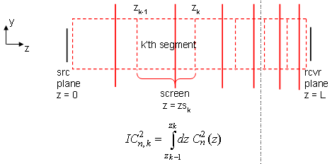
Based on the integrated Cn2 , we define an effective screen Cn2 as the path-averaged value:
( effective screen Cn,k2 ) = ICn,k2 / (zk - zk-1)
Whenever the WaveTrain user employs an input format that requests explicit values of screen Cn2 , the values are interpreted in the effective, or path-averaged sense just defined. In other words, what Wavetrain does is to take an input value of screen Cn2 , and multiply it by the corresponding subinterval length (or screen "thickness") to obtain the integrated quantity that actually determines the screen OPD strength.
Readers who are familiar with optical turbulence theory will realize that ICn2 is closely related to the plane-wave r0 (Fried coherence length) quantity. In fact, WaveTrain has one input format for specifying screen strengths that requests screen-r0 values. Users who are familiar with this way of specifying screen strengths may prefer this input format to the Cn2-based formats.
Position of phase screens within the subintervals
In some WaveTrain input formats, the user can place the individual screens at arbitrary positions within their respective subintervals. The best choice depends on the physical problem being modeled, and the turbulence path-weighting functions that are most important to the problem at hand. Since several different weighting function are often significant in a physical problem, it is not always obvious what the optimum discrete positioning choice is.
In other WaveTrain input formats, the code internally decides where to place the screens within the designated subintervals.
Other phase screen parameters
In addition to the previously discussed strength and position parameters, the phase screen specifications contain numerous optional parameters. Examples are screen transverse velocities, inner and outer scale lengths, and intensity transmission factors. The availability and syntax of various options is documented in the section on the AcsAtmSpec function. The remainder of the present section contains general remarks on several of the options.
Transverse velocities
Transverse velocities associated directly with the screens in the AcsAtmSpec function can be used in two ways. If the velocities of target and platform motion are all specified by using TransverseVelocity library modules, then additional velocities specified explicitly as "screen velocities" should be interpreted as true-wind velocities. WaveTrain will form the appropriate vector sums to obtain the relative motion of the nominal beam line with respect to the air mass.
There is a different approach to handling transverse velocity, which may be preferred by users who have some previous experience with "home-brewed" wave-optics simulation. In many systems, one could dispense with WaveTrain's TransverseVelocity procedures, and simply precompute by hand the effective velocities with which the screens should be dragged, accounting for all target, platform, and true-wind velocities. Then, these net pseudo-wind velocities could simply be inserted as the "screen velocities" in the AcsAtmSpec function. These alternate approaches to handling transverse motion have been discussed at somewhat greater length in previous sections.
Inner and outer scales of turbulence
The optional inner and outer scale roll-offs are modifications to the pure Kolmogorov power-law spectrum of refractive index fluctuations. The functional form and length of the outer scale depends in complicated ways on boundary conditions. Modelers usually use a simple empirical rolloff known as the vonKarmann form, in which the Kolmogorov power law bends over and asymptotes to a constant at low spatial frequency. The break point on a radian frequency scale is (1 / L0), where L0 is called the outer scale (see Andrews and Phillips, pp. 53ff.). If desired, L0 can be specified on a screen-by-screen basis in AcsAtmSpec. In many modeling problems, the outer scale is sufficiently larger than aperture or beam sizes so that L0 is effectively infinite. If no outer scale specification is entered in AcsAtmSpec, it will be treated as infinite.
The inner scale modification of the Kolmogorov power
spectrum is on a firmer theoretical and experimental footing than the outer
scale. When analysts explicitly include inner scale, it is often
represented as a Gaussian rolloff factor at high spatial frequency, of the form
exp[-(K/Km)2], where K is radian spatial frequency, and
the inner scale length is
l0
= 5.92/Km. Although this form is more tractable for
analytic calculations, the modern literature has established that a more
accurate form of the spectral modification is the so-called "Hill bump" form
(see Andrews and Phillips, pp. 53ff.).
In simulation, this functional form can be encoded with little extra trouble,
and this option is available in the AcsAtmSpec
function. If desired, inner scale length can be specified on a
screen-by-screen basis in AcsAtmSpec. If no inner scale is specified, it
will be treated as zero. There is a practical limitation due to the
discrete simulation mesh: the propagation mesh spacing effectively
determines an inner scale even though no explicit factor is entered into the
spectrum formula from which the screens are constructed.
Transmission factors
Screen "transmission" implies intensity transmission to be associated with that screen or subinterval. For most WaveTrain work, the screen transmission options are not used: the library also provides overall transmission-factor modules, so it is unnecessary to decompose the transmission by screen. The exception to this is if the WaveTrain thermal blooming capability is used, but then one must use a different input function anyway (MtbAtmSpec).
WaveTrain library modules used to specify turbulence
The WaveTrain subsystems used to model the optical effects of turbulence are AtmoPath or GeneralAtmosphere. If the user prefers to get WaveTrain subsystems via the "sub-libraries", the two subsystems just named can be found inside the AtmosLib sub-library. As far as turbulence specification is concerned, there is no difference between AtmoPath and GeneralAtmosphere. AtmoPath is a composite system that consists of GeneralAtmosphere plus two PropagationControllers. For new WaveTrain users, we suggest the use of AtmoPath, which simplifies matters by automatically setting certain options. The circumstances under which one wants to separately invoke GeneralAtmosphere and PropagationControllers are discussed in another Guide section.
In the present tutorial section, we explain the turbulence
inputs in the context of the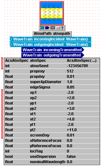 AtmoPath module. The
specifications are essentially the same in
GeneralAtmosphere, when
the user graduates to that level. The diagram at right shows the interface
of AtmoPath. The module has a wavetrain input and a wavetrain output for
each propagation direction. Additionally, there are many parameters, and
the ones directly relevant to turbulence specification are bracketed by the red
bars.
AtmoPath module. The
specifications are essentially the same in
GeneralAtmosphere, when
the user graduates to that level. The diagram at right shows the interface
of AtmoPath. The module has a wavetrain input and a wavetrain output for
each propagation direction. Additionally, there are many parameters, and
the ones directly relevant to turbulence specification are bracketed by the red
bars.
The first parameter, named
atmSpec, has a unique
data type,
AcsAtmSpec. This parameter carries all the
information regarding the turbulence strength and distribution: the number of
phase screens, their locations, strengths, inner scales, outer scales, and so
forth. In the sample at right, this information is entered in a
setting expression
that uses a special function from the WaveTrain library:
AcsAtmSpec(...)
The name of the function should be entered just as shown, and the ellipsis
replaced by a sequence of input arguments that has numerous options.
Several of the most useful argument syntax options of
AcsAtmSpec are documented in detail in the next subsection. From time
to time, new options are added, and the more experienced and bold WaveTrain user
may benefit from inspecting the
source code file that
contains all the options.
The second parameter, atmoSeed, is the random number seed used to initialize the sequence of phase screen statistical realizations. This can be any allowed integer value. This parameter allows the user to exactly reproduce a particular set of turbulence screens: in this way, we can vary some overall system parameters while using exactly the same turbulence realizations.
The next relevant group of parameters stretches from xp1 to yt2. These parameters specify the transverse spans of the phase screens. As the system evolves, there may be relative motion between sources, medium, and sensors, causing the beams to sample different portions of the phase screens. The relative motion of the screens is carried out internally by WaveTrain, based on transverse motion specifications defined by the user. The "rectangular region" (xp1,xp2, yp1,yp2) defines the size of a screen at the platform end (should a screen be exactly at that z), while (xt1,xt2, yt1,yt2) defines the size of a screen at the target end (should a screen be exactly at that z). The indices "1" and "2" here signify "min" and "max", respectively. The sizes of screens at intermediate z locations are determined by linear interpolation from the "rectangular regions" at the two ends. In previous sections on transverse motion, we explained in detail how the transverse motion during the full simulation is used to determine appropriate values for the screen "rectangular regions". The numerical values entered as setting expressions in the above picture derive from an example discussed in that previous section. The link just referenced should be reviewed in conjunction with the present one for full coverage of phase screen specifications.
The final turbulence parameter is screenDxy. This is the mesh spacing of the phase screens. We have set this spacing equal to the propdxy value, which is a typical choice, though not obligatory. Based on screenDxy, WaveTrain may make some adjustment to the screen size because of FFT (Fast Fourier Transform) constraints. For example, to determine one of the actual dimensions of the phase screen mesh, (xp2-xp1)/screenDxy will be rounded up to the nearest convenient integer for the FFT routines, so that the screens will usually be somewhat bigger than the user specifications (xp1,...).
Use of AcsAtmSpec to specify turbulence parameters and path geometry
To enter turbulence specifications into a WaveTrain simulation, one uses the AcsAtmSpec function in a setting expression in AtmoPath or GeneralAtmosphere. The mechanism was illustrated in the first parameter line in the preceding picture. AcsAtmSpec has many different allowed sets of arguments. (At the C++ code level, these options are referred to as different "constructors" or initialization functions.) The following table documents several of the most useful syntax options. From time to time, between official WaveTrain releases, new options are added by WaveTrain programmers to handle new special cases that are judged convenient or necessary. The more experienced and bold WaveTrain user may benefit from inspecting the source code file that contains all the options. After some of the cases documented below have been digested, the user can probably understand the multitudinous other allowed formats by inspecting the argument lists in the referenced source code file.
General rules
There are some general rules that apply to all argument list options (or at least to all cases where the item appears):
(1) In the table below, the data types of the arguments are prefixed to the arguments. The purpose of doing this in the table is just to clarify whether the arguments are scalars or vectors: when the user actually enters the setting expression in WaveTrain, the data type designators should be omitted.
(2) Argument lambda
refers to a reference wavelength.
CAUTION: the wavelength in question here may be, but is not
necessarily, the wavelength of the propagating beam. In the listed
syntax options where it appears, lambda
is the
reference wavelength at which the r0s of the screens are defined.
The effective r0 of a screen will then depend on the propagating wavelength, but
we want to define the screens only once, at some reference wavelength.
(3) Argument pathLength refers to the total propagation range from platform end to target end of the atmospheric module. Note that screens are not necessarily located at the endpoints, so pathLength is frequently greater than the distance between first and last screens.
(4) The positions (z coordinates) of screens are defined with respect to WaveTrain's z-coordinate conventions. The key facts are that z=0 is the platform end and z=L(propagation range) is the target end of the atmospheric propagation module into which AcsAtmSpec is inserted.
(5) Arguments that specify inner and outer scales, screen
velocities, and screen transmissions have obvious default values. The
defaults are: inner scale = 0.0, outer scale = infinity, velocities
= 0.0, and transmissions = 1.0.
To obtain the default values, the user should simply omit these arguments from
the setting expression. BUT, note that only a contiguous set of
trailing arguments in a list may be omitted.
"Transmission" here implies intensity transmission to be associated with
that screen or subinterval. For most WaveTrain work, the screen
transmission options are not used, because the library also provides overall
transmission-factor modules.
(6) Some syntax options have height specifications, usually encoded as hPlatform and hTarget. In these cases the user can specify the turbulence strength in terms of a named turbulence profile, such as Clear-1, Clear-2, or HV57. In these cases, h should be interpreted as height above mean sea level (AMSL), because the named Cn2 profile options such as "Clear-1" have their Cn2(h) functional forms defined in terms of height AMSL. Additionally, when using the named profiles, the user must understand that the Clear-1 and Clear-2 profile functions are only defined for h ≥ 1230 m AMSL, where that height represents (approximately) the ground level altitude at the site where Clear-X data was collected. If the user wishes to apply Clear-X to a physical problem where the ground altitude is different, then a reasonable approach would be to enter h_AMSL values into WaveTrain such that the altitude above ground level is preserved between the physical problem and the simulation specs.
(7) Particularly in the case of vector arguments, the user
will find it most convenient to enter symbolic names for the arguments, elevate
the arguments up the system hierarchy, and
assign values to the vectors at that
top level (i.e., in the Run Set Editor (TRE)).
Actually, this holds for most scalar arguments as well: the atmospheric
specifications in general are quantities that we often wish to vary when
exploring performance, so it is best to elevate those quantities to the Run Set
level before assigning numerical values.
(8) As elsewhere in WaveTrain, physical units are MKS, unless explicitly specified otherwise.
| Usage Case | Setting Expression for atmSpec | |
| 1 | General screen positions and strengths, with strengths expressed as screen-r0 values |
AcsAtmSpec(float lambda, float pathLength, Vector<float> positions, Vector<float> screenr0s, Vector<float> vxs, Vector<float> vys, Vector<float> l0is, Vector<float> l0os, Vector<float> transmissions) *************** Notes: positions = z-coordinates of the screens. vxs, vys = x,y velocity components of screens. l0is = inner scales; l0os = outer scales. Default values for transmissions are 1.0. |
| 2 | General screen positions and strengths, with strengths expressed as screen-Cn2 values |
AcsAtmSpec(float lambda, Vector<float> positions, Vector<float> screenCn2s, Vector<float> thicknesses, float pathLength, float l0i, float l0o, float vX, float vY) *************** Notes: screenCn2s are the effective Cn2 discussed above, thicknesses are the subinterval widths associated with them, and positions are the z-coordinates of the screens. In contrast to the previous syntax option, the inner/outer scale and screen velocities, if used, must be the same for all screens. |
| 3 | Named Cn2 profile, with uniformly-spaced screens |
AcsAtmSpec(int profileNumber, float lambda, int nScreens, float turbFactor, float hPlatform, float hTarget, float pathLength, float l0i, float l0o, float vX, float vY) *************** Notes: profileNumber: 1Þ Clear-1; 2Þ Clear-2; 3Þ HV57. The first screen is placed at z=0, the screen spacing is dz=pathLength/nScreens, and the last screen is at z=(pathLength - dz). turbFactor is an arbitrary uniform multiplier that may be applied to the profile Cn2 strength. CAUTION (see item (6) in the General Rules
above): Clear-1 and -2 profile functions are only defined for h≥1230m,
where that number is approximately the ground altitude above mean sea level
at the geographic site where Clear-X data was collected. |
| 4 | Scaled Clear-1 profile, with uniformly-spaced screens |
AcsAtmSpec(float lambda, int nScreens, float clear1Factor, float hPlatform, float hTarget, float pathLength, float l0i, float l0o, float vx, float vy) *************** Notes: essentially same as previous syntax option 3, but restricted to only the Clear-1 profile, scaled by the uniform multiplier clear1Factor. CAUTION (see item (6) in the General Rules above): The Clear-1 profile function is only defined for h≥1230m, where that number is approximately the ground altitude above mean sea level at the geographic site where Clear-1 data was collected. |
| 5 | Read turbulence parameters from a file with syntax generated by TurbTool |
AcsAtmSpec(char*
filename, float Cn2factor) *************** Notes: This syntax is primarily meant for loading turbulence and configuration data generated by TurbTool, which is a WaveTrain helper application. TurbTool is a Matlab GUI application, and generates *.mat () files. However, the user could also independently generate data files with the right content format and read those. |
| 6 | Read turbulence parameters from a file with syntax generated by PropConfig |
PropConfigAtmSpec(char*
filename) *************** Notes: This syntax is primarily meant for loading turbulence and configuration data generated by PropConfig, which is a WaveTrain helper application. PropConfig is a Matlab GUI application, and generates *.mat () files. However, the user could also independently generate data files with the right content format and read those. CAUTION: notice that the present syntax for the setting expression uses a different function name than all the other syntaxes: "PropConfigAtmSpec" instead of "AcsAtmSpec". |
Phase screen generation and execution time
Phase screen generation is done once, at the beginning of a simulation run. For all subsequent time steps of the simulation run, the existing screens simply shift relative to sources and receivers. This means that quite large screens can be used without much impact on the overall simulation wall-clock time, which is usually dominated by the Fresnel propagations. If multiple runs (each with a different realization of the atmospheric screens) are included in a run set, then of course screens must be generated at the beginnning of each run. The extreme case would be if a run set is constructed from N completely independent realizations, with only one time index per realization: in this case, the phase screen construction could dominate the execution time. The earlier introduction to modeling transverse motion expanded on some of these issues.
Some phase screen construction details
In the previous discussion of determining the size of phase screens, we alluded to a second reason for making "oversize" screens. We briefly discuss this second reason now. A phase screen is a discrete, finite-span statistical realization of a 2-D random process that obeys a specified power spectral density law. Currently, the standard WaveTrain library method of generating screens is the PSD-conditioned white-noise method. The steps of this procedure are: (a) use a standard random-number generator to create an uncorrelated (white) noise random process in the spatial-frequency domain; (b) multiply that by the square root of the theoretical power spectral density (PSD); (c) apply a suitably normalized discrete Fourier transform to obtain the space-domain realization of the correlated random process. A consequence of this algorithm is that the random process it generates is periodic in both dimensions: each edge matches up smoothly with the opposite edge. This has an advantage, in that it makes endless scrolling of the screens possible, but it also means that there can be no overall phase tilt across the screen, which is physically incorrect. In general, other lower-order spatial frequency modes, not just tilt, will also have less power than they should.
Low-order correction option ("locflag" in AtmoPath)
The low-order deficiency just described is often not serious, for several reasons. First, it is typically practical to generate screens that are much bigger than the simulation apertures. As discussed previously, we usually want to generate oversize screens anyway because of relative motion considerations. In this case, the tilt across the receiver aperture distance can be fairly well represented. Secondly, for closed-loop adaptive optics systems, the lowest-order modes are the easiest to compensate, so one might argue that it is not very important to model them exactly.
On the other hand, to get accurate low-order results for
uncompensated systems, users may want to invoke a modified screen-generation
technique that
AtmoPath makes available.
Inspection of AtmoPath's parameter list shows a parameter called
locFlag, where "loc"
stands for "low-order correction". The default setting is
locFlag = 0, which leaves the
PSD-conditioned white-noise screens unchanged. But, setting
locFlag = 1 invokes a
calculation that separately computes realizations of several low-order modes,
and inserts a corresponding compensation into the phase screens that will be
used for optical propagation.
Atmospheric modeling using TurbTool or PropConfig
We must always use the AcsAtmSpec function to input turbulence information into WaveTrain. As explained in the preceding section covering AcsAtmSpec usage, some syntax options of AcsAtmSpec generate the required screen-Cn2 values internally, but other syntax options require the user to independently provide the effective Cn2 or screen-r0 values along the propagation path. For some model building, it may be simple for the user to generate these numbers independently. On the other hand, there may be significant work involved in generating the numbers, particularly if one wants to explore different scenarios with named atmospheric turbulence profiles like Clear-1, HV57, SLC, AMOS, etc.
As a separate issue, in conjunction with setting up a WaveTrain model, users will usually want to carry out auxiliary calculations using "well-known", albeit approximate, closed-form formulas from basic turbulence theory. We have in mind tasks like calculating the scintillation index (log-amplitude or normalized intensity variance), Fried's r0, or Greenwood frequency for the propagation path of interest.
The WaveTrain code suite contains two helper applications that can assist users with the above issues and others. These helper applications are Matlab programs, whose graphical user interfaces (GUIs) must be started at a Matlab prompt (i.e., outside of WaveTrain). In WaveTrain versions 2009A and earlier, there was one helper application, called TurbTool. In WaveTrain version 2010A, there are two separate applications, called TurbTool and PropConfig, respectively. In future WaveTrain versions, TurbTool will be phased out in favor of PropConfig. PropConfig is a reworked version of Turbtool, which can do essentially everything that TurbTool does, and also has significant additional capabilities. MZA will continue to support TurbTool for the present, for the benefit of existing users. However, new users should learn PropConfig, and ignore TurbTool.
TurbTool and PropConfig can be used completely independently of WaveTrain (e.g., to simply compute integrated-turbulence quantities), or they can be used in conjunction with WaveTrain, to generate input vectors for the WaveTrain AcsAtmSpec function and/or to approximately scope out a problem that will be explored in detail by WaveTrain.
In brief, TurbTool or PropConfig can assist WaveTrain users as follows:
(1) The user can generate vectors of effective Cn2 or screen-r0 values, which can then be easily copied manually into a WaveTrain run set. The values are based on user-selectable atmospheric models: standard profile models such as HV5/7, CLEAR-1 and others are available.
(2) As an alternative to the manual transfer in (1), the application can write a data file whose name can later be supplied to one of the AcsAtmSpec syntax options in the above table of cases.
(3) The user can quickly compute analytic estimates of certain important integrated-turbulence quantities, such as normalized irradiance variance or full-path r0, for a variety of propagation paths of interest. This may be very helpful for comparison with the wave-optics results, or for general orientation. In the latter sense, TurbTool or PropConfig can be used completely independently of WaveTrain.
(4) The user can generate vectors of absorption and scattering coefficients to associate with phase screens, in order to specify position-dependent attenuation and absorption. The absorption component would be relevant if thermal blooming is included in the WaveTrain simulation. The numerical values are based on the validated MODTRAN and FASCODE codes developed at the Air Force Geophysics Laboratory, supplemented by other specialized models.
(5) [PropConfig only]: the application can generate suggested propagation mesh parameters (spacing and point dimension) for use by WaveTrain's numerical Fresnel propagation modules.
Use of TurbTool or PropConfig is not required to have full WaveTrain functionality, but most users will find the applications helpful for at least one of the functions outlined above.
Use of TurbTool (available in WaveTrain 2010A and earlier versions)
To use TurbTool, the start procedure is:
(1) Open a Matlab session.
(2) In more recent versions of WaveTrain, the installer should have already set the necessary Matlab paths. Try skipping to step (3), and see if the TurbTool main screen (shown below) appears.
If Turbtool did not start, do the following manually:
Make the current directory
(3) At the Matlab prompt, type:
>> turbtool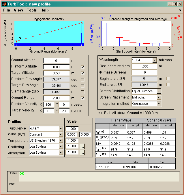
Use of PropConfig (available in WaveTrain 2010A and later versions)
To use PropConfig, the start procedure is:
(1) Open a Matlab session.
(2) The WaveTrain installer should have already set the necessary Matlab paths to access the PropConfig functions.
(3) At the Matlab prompt, type:
>> PropConfig
(4) Depending on installed versions of certain graphics support libraries,
the text and numbers of graphics panels in the PropConfig screen may display
improperly. If you observe display problems, try the following:
a) exit from PropConfig
b) at the Matlab prompt, type
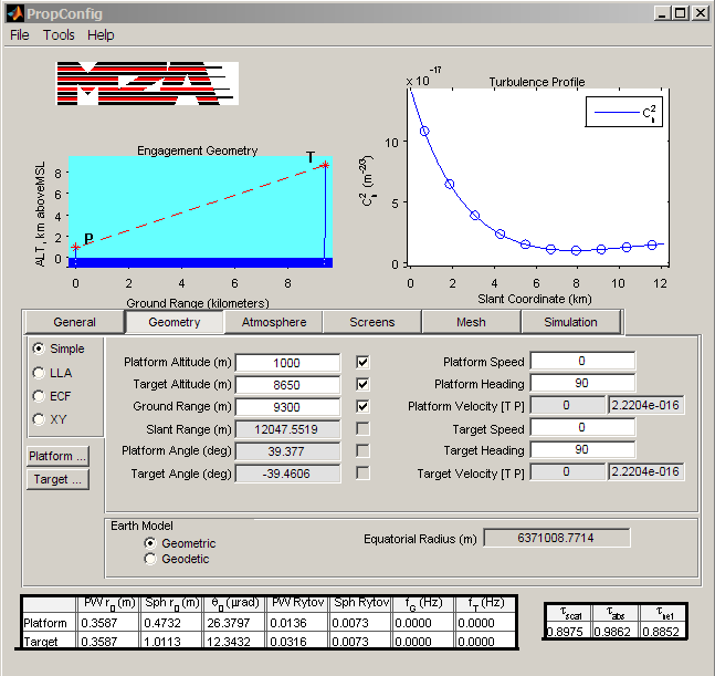
Using atmospheric thermal blooming models
RESTRICTED AVAILABILITY NOTICE:
The thermal-blooming components of WaveTrain are only available with specific
permission from the government sponsor. Contact MZA Associates for
details.
In addition to atmospheric turbulence, there is another physical phenomenon that can add further distortion to the phase front of a propagating optical beam. This new distortion is due to heating of the medium caused by absorption of part of the beam energy. The numbers are such that, generally, this phenomenon is only noticeable in atmospheric propagation with truly high-energy lasers. The heating of the medium is spatially non-uniform, due to finite-beam geometry as well as turbulence scintillation. Consequently, there are non-uniform density changes in the medium, which produces a non-uniform refractive index field, which in turn produces new phase distortions upon propagation. From its manifestation in a simple geometry, the beam distortions due to the heating are known as "thermal blooming".
To numerically simulate the effect of thermal blooming on wave-optics propagation, we use a procedure that meshes with the split-step method described earlier for modeling the effect of turbulence. The propagation path is again divided into subintervals, and the integrated phase retardation map for that subinterval is computed. From this, a blooming phase screen is constructed, and then used in the framework of the split-step propagation concept. Typically, there will be turbulence phase screens in addition to blooming phase screens, although one can of course set the turbulence strength to zero to study the blooming effect in isolation.
Since atmospheric absorption is the source of thermal blooming, evidently the key new physical information that must be supplied is a profile of atmospheric absorption coefficients along the propagation path, together with allied information. Since the absolute power or energy striking each screen determines the heating in the associated subinterval, a profile of atmospheric scattering coefficients is required in addition to the absorption coefficients. Only the absorbed energy translates into heating, but scattering reduces the net beam power and hence reduces the absolute amount of energy absorbed for a given absorption coefficient. The scattered energy simply disappears from the problem in the WaveTrain model.
The WaveTrain setup procedures for a system with thermal
blooming parallel the setup procedures for a system with turbulence only.
The key differences are that we:
(1) Use the components TBAtmoPath or
TurbBloomAtmosphere instead of AtmoPath
or GeneralAtmosphere.
(2) Use the function MtbAtmSpec in addition to
AcsAtmSpec. (AcsAtmSpec is still used to specify
the turbulence screens and specs).
Acknowledgement
The computer code for creating the thermal blooming phase screens in WaveTrain was copied directly from the MOLLY code created by authors at the MIT Lincoln Laboratory. The key portions of the MOLLY code were integrated into the WaveTrain propagation framework.
WaveTrain library modules used to specify thermal blooming
The WaveTrain subsystems used to model thermal blooming in conjunction with turbulence are TBAtmoPath or TurbBloomAtmosphere. These two modules play the same role as AtmoPath or GeneralAtmosphere, respectively, play for turbulence alone. Note that TBAtmoPath and TurbBloomAtmosphere contain both thermal blooming and turbulence specifications, so they can be used instead of, not in addition to, AtmoPath or GeneralAtmosphere.
TBAtmoPath and TurbBloomAtmosphere are related to each other in the same way that AtmoPath and GeneralAtmosphere are related. TBAtmoPath is a composite system that consists of TurbBloomAtmosphere plus two PropagationControllers. For new WaveTrain users, we suggest the use of TBAtmoPath, which simplifies matters by automatically setting certain options. The circumstances under which one wants to separately invoke PropagationControllers are discussed in another Guide section.
In the present tutorial section, we explain the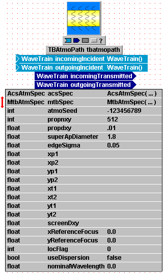 turbulence inputs in the context of the
TBAtmoPath module. The
specifications are essentially the same in
TurbBloomAtmosphere,
when the user graduates to that level. The diagram at right shows the
interface of TBAtmoPath. The module has a wavetrain input and a wavetrain
output for each propagation direction. Additionally, there are many
parameters, but only the one bracketed by the red bar is specifically relevant
to thermal blooming. The remaining parameters are the same ones that
appeared in the AtmoPath interface, and
specify the turbulence-related parameters. The new parameter is named
mtbSpec, and its setting
expression is used to enter all the data needed for thermal blooming
specifications. In the sample at right, this information is entered in a
setting expression
that uses a special function from the WaveTrain library:
turbulence inputs in the context of the
TBAtmoPath module. The
specifications are essentially the same in
TurbBloomAtmosphere,
when the user graduates to that level. The diagram at right shows the
interface of TBAtmoPath. The module has a wavetrain input and a wavetrain
output for each propagation direction. Additionally, there are many
parameters, but only the one bracketed by the red bar is specifically relevant
to thermal blooming. The remaining parameters are the same ones that
appeared in the AtmoPath interface, and
specify the turbulence-related parameters. The new parameter is named
mtbSpec, and its setting
expression is used to enter all the data needed for thermal blooming
specifications. In the sample at right, this information is entered in a
setting expression
that uses a special function from the WaveTrain library:
MtbAtmSpec(...)
The name of the function should be entered just as shown, and the ellipsis
replaced by a sequence of input arguments.
As noted above, the single library module TBAtmoPath is used to specify both the turbulence and the thermal blooming data. The parameters other than mtbSpec have the same meaning for turbulence as explained in the section describing the AtmoPath module.
Use of MtbAtmSpec to specify blooming parameters and path geometry
To enter thermal blooming specifications into a WaveTrain simulation, one uses the MtbAtmSpec function in a setting expression in TBAtmoPath. The mechanism is illustrated in the second parameter line in the preceding picture. In the same vein as AcsAtmSpec, MtbAtmSpec has several different allowed sets of arguments. The following table of cases illustrates several options. After digesting the cases documented below, the more experienced user can inspect the argument lists in the source code file to see if other options may be useful. The available options may be increased from time to time, between official releases of WaveTrain.
General rules
There are some general rules that apply to all argument list options (or at least to all cases where the item appears):
(1) In the table below, the data types of the arguments are prefixed to the arguments. The purpose of doing this in the table is just to clarify whether the arguments are scalars or vectors: when the user actually enters the setting expression in WaveTrain, the data type designators should be omitted.
(2) The position (z) coordinates of screens, are defined with respect to WaveTrain's z-coordinate conventions. The key facts are that z=0 is the platform end and z=L(propagation range) is the target end of the propagation module into which MtbAtmSpec is inserted.
(3) Particularly in the case of vector arguments, the user
will find it most convenient to enter symbolic names for the arguments, elevate
the arguments up the system hierarchy, and
assign values to the vectors at that
top level (i.e., in the Run Set Editor (TRE)).
Actually, this holds for most scalar arguments as well: the atmospheric
specifications in general are quantities that we often wish to vary when
exploring performance, so it is best to elevate those quantities to the Run Set
level before assigning numerical values.
(4) As elsewhere in WaveTrain, physical units are MKS, unless explicitly specified otherwise. In particular, absorption and scattering coefficients should have units of m-1. However, temperature should be in °C (note: not Kelvin).
| Usage Case | Setting Expression for mtbSpec | |
| 1 | General atmospheric absorption and scatter coefficient profiles |
MtbAtmSpec(int nxy, float dxy, float xmin, float ymin, float dtime, Vector<float> absorption, Vector<float> scatter, Vector<float> temperature, float lambda, Vector<float> positions, Vector<float> xWind, Vector<float> yWind, float xvs, float yvs, float xvt, float yvt, int numberSavedStates) *************** Notes: See below table for parameter definitions. |
| 2 | Uniform atmospheric absorption and scatter coefficient profiles |
MtbAtmSpec(int nxy, float dxy, float xmin, float ymin, float dtime, float absorption, float scatter, float temperature, float lambda, Vector<float> positions, Vector<float> xWind, Vector<float> yWind, float xvs, float yvs, float xvt, float yvt, int numberSavedStates) *************** Notes: See below table for parameter definitions. |
| 3 |
MtbAtmSpec(int nScreens) *************** Notes: nScreens must be equal to the number of turbulence phase screens.
|
|
| 4 | Read parameters from a file (primarily, a file generated by TurbTool) |
MtbAtmSpec(char*
filename, int nxy, float dxy) *************** Notes: This syntax is primarily meant for loading data generated by TurbTool, which is a WaveTrain helper application. TurbTool is a Matlab GUI application, and generates *.mat () files. |
| 5 | Read parameters from a file (primarily, a file generated by PropConfig) |
PropConfigTBAtmSpec(char*
filename, int nxy, float dxy) *************** Notes: This syntax is primarily meant for loading data generated by PropConfig, which is a WaveTrain helper application. PropConfig is a Matlab GUI application, and generates *.mat () files. CAUTION: notice that the present syntax for the setting expression uses a different function name than all the other syntaxes: "PropConfigTBAtmSpec" instead of "MtbAtmSpec". |
Definition of parameters in table of cases
nxy – the number of points across the thermal blooming screen (currently this is assumed to be a square lattice of points).
dxy – the spacing between adjacent points in the thermal blooming screen (measured in meters).
xmin – x-coordinate of the lower left hand corner of the thermal screen (this is currently setup to match the lower left hand corner of the propagation mesh).
ymin – y-coordinate of the lower left hand corner of the thermal screen (this is currently setup to match the lower left hand corner of the propagation mesh).
dtime – time delta between successive updates of the thermal screens (should be set to the record time of the output at the target end of the propagation, measured in seconds).
absorption – the absorption portion of the extinction (measured in meters-1).
scattering – the scattering portion of the extinction (measured in meters-1).
temperature – representative of the ambient temperature in the temperature model implemented (in degrees centigrade).
lambda – the wavelength (in meters) of the HEL (high-energy laser beam), which creates the thermal screens. Currently the model supports only one HEL beam. .
positions – specifies the distance of the thermal screens from the HEL beam’s aperture (in meters). CAUTION: there is presently a special constraint on the screen positions: see the two worked examples in a linked document.
xWind – specifies the velocity of the true wind in the x-direction at each of the thermal screens (measured in meters/second).
yWind – specifies the velocity of the true wind in the y-direction at each of the thermal screens (measured in meters/second.)
xvs – the slew speed in the x-direction (conforms to WaveTrain notation rate-of-change-in-x-slope).
yvs – the slew speed in the y-direction (conforms to WaveTrain notation rate-of-change-in-y-slope).
xvt – the translation speed in the x-direction of the platform relative to the atmosphere (measured in meters/second).
yvt – the translation speed in the y-direction of the platform relative to the atmosphere (measured in meters/second.)
numberSavedStates – specifies the number of past thermal screens that are required. While for most applications, a value of one for this parameter suffices, it may occur in simulations involving very long propagation paths that past thermal states are needed to accurately model the return from a target. An example of its use is provided in the sample problems.
Sample Problems
Due to the complexity of the parameter setup for thermal blooming, it may be helpful for the user to have some examples and sample results for reference. Two worked examples are given in an auxiliary document.
Use of TurbTool or PropConfig to generate blooming parameters and path geometry
As illustrated in the above table of basic cases, we must always use either the MtbAtmSpec or the PropConfigTBAtmSpec functions to input thermal blooming information into WaveTrain. Depending on the data possessed by the user, it may be simple to create the required input numbers for MtbAtmSpec. However, just as in the case of the AcsAtmSpec input data, the user may find it helpful to obtain absorption and scattering coefficient data by doing preliminary work with the TurbTool or PropConfig helper programs.
Basic sensor modules: TargetBoard, SimpleFieldSensor and Camera
Three fundamental sensor modules provided in the WaveTrain library are TargetBoard, SimpleFieldSensor, and Camera. In the present section we concentrate on TargetBoard and SimpleFieldSensor, but we also describe several important properties common to all three basic sensors, as well as to more specialized WaveTrain sensors.
The following picture shows the interfaces of TargetBoard and SimpleFieldSensor. The interfaces are essentially identical; the principal difference is that TargetBoard outputs the integrated intensity incident at the sensor, while SimpleFieldSensor reports integrated complex field incident at the sensor. As defined in the linked sections, the "integrated" in these two terms refers to temporal integration.
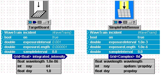
All of WaveTrain's sensors are of the temporally integrating type, based on the specification of an exposure length. The output variable in TargetBoard, called integrated_intensity, has the physical units of J/m2. If the user is more interested in the irradiance, W/m2, that number must obtained by dividing out the exposure length in post-processing. In the case of SimpleFieldSensor, the integrated complex field output (called simply fld in the interface) is somewhat eccentric: this quantity was explained in an earlier section on WaveTrain nomenclature.
As we see from the above picture of the module interfaces, these (and other) WaveTrain sensors have a common set of timing inputs: on, exposureInterval, exposureLength, and sampleInterval. These quantities have the same function in all the sensors, and their usage was explained in the section on timing and triggering.
Wavelength sensitivity
As the picture shows, the first parameter in TargetBoard and SimpleFieldSensor specifies the single wavelength to which the sensor responds. If light of a different wavelength impinges on the sensor, zero signal will be reported by the sensor. Note that some of WaveTrain's other sensor modules have a slightly different wavelength interface: e.g., Camera allows the user to specify a minimum and maximum wavelength of response. In this connection, note also that the WaveTrain library provides a number of spectral filter components. However, the filter components are often unnecessary because of the wavelength selectivity built into the sensor interfaces.
Multiple beams incident on sensor, interference
If the wavetrain incident on a sensor contains beams from two or more sources, of wavelengths to which the sensor responds, then the reported output is a sum of type consistent with the physical nature of the sensor output. Specifically, intensity sensors such as TargetBoard and Camera will add the individual integrated intensities, while SimpleFieldSensor will add the individual integrated complex fields.
If we wish to model the interference of two (or more) beams from sources that are temporally coherent, then we may need some special measures. We consider two cases. First, the interference between coherent beams of identical wavelength is easy to model. We must use SimpleFieldSensor to compute the complex field superposition, and then in post-processing take the squared magnitude of the net output if that is the quantity of interest.
The second case of interest occurs if the incident beams have different wavelengths but are still temporally coherent. In that case, the field superposition created by SimpleFieldSensor only has meaning if the system includes special modeling provisions: see the section on interference of polychromatic fields.
Spatial sampling, integration and interpolation
The remaining parameters in the interface specify the mesh (nxy,dxy) on which sensor output is reported. The mesh registration for TargetBoard and SImpleFieldDensor is of "gwoom" type, and nxy may be even or odd. Note the mesh parameters only provide for square sensors. An asymmetric sensor could be constructed as a composite subsystem by relatively displacing a set of square sensors. The other option of course is simply to ignore the zeros reported by the sensor outside an asymmetric region of interest: in practice, this is usually an adequate procedure.
It is important to understand that the output of all sensor modules represents point samples, at the sensor mesh points, of whatever physical quantity the sensor reports. For example, suppose that a TargetBoard dxy specification is two times the propagation mesh dxy of the incident field. In that case, the sensor performs no spatial integration or smoothing of the incident field: the sensor simply reports point samples seen at its own (nxy,dxy) mesh. If the mesh points are not precisely registered because of transverse displacements (e.g., motion-induced), then the sensor modules will automaticaly do nearest-neighbor interpolation to best estimate the point samples. Of course, to model practical situations it may be important to introduce the modeling of spatial integration that is performed by physical sensor pixels that are large compared to the spatial intensity or field variation that is incident on the sensor. To perform such calculations, the WaveTrain library provides spatial integration capabilities in a module called (somewhat inaptly) SensorNoise.
Camera,
whose interface is shown at right, is the third basic senso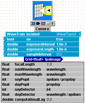 r
module. Camera ultimately outputs a quantity of the integrated intensity
type. Important properties of Camera concerned with timing inputs,
wavelength selectivity, multiple incident beams, spatial sampling and
integration follow the principles discussed in the
basic sensors overview. In the
present section, we focus on the unique properties of Camera. Camera is
more complicated than the previously discussed TargetBoard and
SimpleFieldSensor, since Camera has two significant planes, namely an aperture
and a sensor plane. Note that in the Camera interface names, "detector"
refers to "sensor" plane.
r
module. Camera ultimately outputs a quantity of the integrated intensity
type. Important properties of Camera concerned with timing inputs,
wavelength selectivity, multiple incident beams, spatial sampling and
integration follow the principles discussed in the
basic sensors overview. In the
present section, we focus on the unique properties of Camera. Camera is
more complicated than the previously discussed TargetBoard and
SimpleFieldSensor, since Camera has two significant planes, namely an aperture
and a sensor plane. Note that in the Camera interface names, "detector"
refers to "sensor" plane.
Sensor-plane parameters
In general terms, Camera forms a far-field image from the complex field incident on the module. Camera is characterized optically by its focalLength parameter. Based on the focal length value, Camera computes the complex field and then the intensity that is formed in the focal plane. More precisely, Camera takes the incident complex field, computes its space-domain Fourier transform, and outputs (const · |transform|2). The factor (const) is constructed so that the output is the physical integrated intensity (J/m2) in the focal plane. The output variable is called fpaImage (fpa = focal-plane array), and the transverse mesh on which its values are reported is defined by the parameters (nxyDetector, dxyDetector).
The significance of the (nxyDetector, dxyDetector) specification is tricky. The transverse scale of fpaImage is determined by the focalLength parameter, as follows. The complex field incident on Camera exists on the full propagation mesh (even though some values may be zeroed out by a preceding aperture): let the propagation mesh parameters be (nxyprop, dxyprop). Now, regardless of the (nxyDetector, dxyDetector) specs, the mesh spacing on which Camera's Fourier Transform result is internally computed is:
dxy_FT = [wavelength/(nxyprop·dxyprop)] · focaLength
Equivalently stated, a Discrete Fourier Transform operation is applied to the complex field on the entire incident mesh, and the result exists on a mesh whose parameters are (dxy_FT, nxyprop). Now, if we set the interface parameter dxyDetector = dxy_FT, then we would exploit the full available resolution of the Camera calculation. If desired, the user can subsample that result by setting dxyDetector to a coarser spacing than dxy_FT. Whether the user wants to subsample or not will usually depend on the dimension of the physical aperture that is placed in front of Camera. This physical aperture is discussed next.
CAUTION: dxyDetector in Camera has the following potentially confusing aspect. If dxyDetector is coarser than dxy_FT, then WaveTrain's reported fpaImage values are simply point-interpolated from the original |transform|2 values on the dxy_FT mesh. This is NOT equivalent to spatially integrating the irradiance over physical pixels whose size is dxyDetector. Depending on the physical system, such a spatial integration may be critical to a physically valid model of camera output. Spatial integration of that sort must be accomplished with an extra WaveTrain component.
Defining the aperture for Camera, and adjusting the image plane
CAUTION: another potentially confusing aspect of the Camera (and certain other imaging sensors, like HartmannWfsDft), is the interface parameter pair (nxyPupil, dxyPupil). From their names, one might think that these parameters actually specify a camera pupil size, but that is NOT the meaning. These two parameters are only used in conjunction with the technique of "wavesharing", which is an advanced option that attempts to eliminate redundant propagations that can occur in WaveTrain when multiple sensors are present. (We recommend that users become very familiar with WaveTrain before attempting to use wavesharing.) Unless wavesharing is being used, the parameters (nxyPupil, dxyPupil) have absolutely NO effect. However, even if not used, they must be assigned some arbitrary numerical values, because all parameters and inputs must be assigned values.
In order to define the physical entrance pupil (aperture) for a Camera module, the user must insert an Aperture or related module in front of the Camera. For a reason to be explained now, the Telescope module is frequently used for this purpose. The following illustration shows, in the top panel, the interface of Telescope, and in the lower panel, the contents of Telescope.
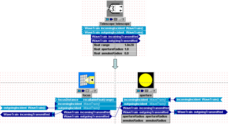
We see that Telescope consists of an Aperture module and a Focus module. In the present context, the purpose of the Focus module is to compensate for the fact that the source of the wave being imaged by Camera may be at some finite distance instead of infinity. The Fourier Transform computation of Camera, with the focalLength specified in Camera, gives the field in the focal plane corresponding to the field in the entrance plane of the Camera module. Typically (though not always) what is wanted as the Camera output is the intensity in the image plane of the source. Therefore, we must add an extra (usually small) focus increment in order to make the image plane of the net system (Focus + Camera) coincide with the focal plane of Camera. This is achieved if we set the range parameter in Telescope equal to the object distance. The clearest way of understanding this is that a Telescope focus equal to the object range will collimate a point source located at the object: subsequently, this collimated wave entering Camera is focused at the focal plane of Camera, which means that the focal plane of Camera is now the image plane of the source. The user can of course insert separate Aperture and Focus modules to achieve the purpose described here, but the Telescope system provides a convenient combination module.
Spatially integrating WaveTrain sensor outputs
In the section on basic properties of sensor modules, we explained that the WaveTrain sensors all provide point samples on the specified detector mesh. If the field incident on the detector mesh plane has significant spatial variations, and if the physical pixel size to be modeled does not resolve those variations, then it is usually necessary to perform spatial integration over the physical pixel size in order to obtain the desired modeling result. The WaveTrain library system provided for that purpose is called SensorNoise. The name may seem inappropriate, but this system does double duty: the optional addition of various kinds of detection noise is a second capability of this module. The following diagram shows the interface of SensorNoise:
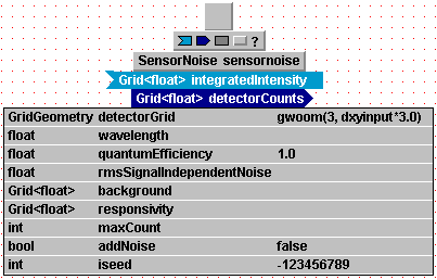
As we see in the interface picture, the input to SensorNoise is assumed to be an integrated intensity: this will usually be the output of one of WaveTrain's intensity-sensor modules, such as TargetBoard, Camera, or HartmannWfsDft. The output of SensorNoise, called detectorCounts, will be in units of digital counts. At the end of the present section, we make some remarks regarding the units conversion, but our immediate focus is on the spatial integration feature.
The basic concept used by SensorNoise to set up the
spatial integration is the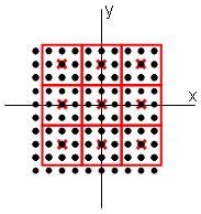 specification of a new mesh, whose points represent the centers of the physical
pixels. This new mesh is specified by the parameter
detectorGrid. A
concrete example may be helpful. In the diagram at right, there is mesh
indicated by black dots. Suppose this is the output mesh of a TargetBoard
or Camera module, and that this is the mesh on which SensorNoise's input
integratedIntensity is given.
Next, suppose that we are interested in the response of a physical sensor whose
pixel width is three times the black-dot mesh spacing. The boundaries of
the physical pixels are indicated by the red lines. In order to specify
these physical pixels to WaveTrain, we must define the
detectorGrid mesh to be the
center points shown as red crosses. Since the
detectorGrid parameter has
data type "GridGeometry" (see column 1 of the
parameters list), we must use one of several special WaveTrain
library functions to define the new mesh.
In the above picture of the SensorNoise interface, we have entered a
setting expression that uses the "gwoom" function:
gwoom(3,dxyinput*3.0). The first function
argument signifies the mesh dimension of the new mesh, and the second argument
signifies the mesh spacing of the new mesh. (The symbol
dxyinput would have to be elevated or replaced locally
by a number.) For further background and all the options for mesh
specification, see the introduction to meshes
and the detail section on the functions gwoom and
GridGeometry.
specification of a new mesh, whose points represent the centers of the physical
pixels. This new mesh is specified by the parameter
detectorGrid. A
concrete example may be helpful. In the diagram at right, there is mesh
indicated by black dots. Suppose this is the output mesh of a TargetBoard
or Camera module, and that this is the mesh on which SensorNoise's input
integratedIntensity is given.
Next, suppose that we are interested in the response of a physical sensor whose
pixel width is three times the black-dot mesh spacing. The boundaries of
the physical pixels are indicated by the red lines. In order to specify
these physical pixels to WaveTrain, we must define the
detectorGrid mesh to be the
center points shown as red crosses. Since the
detectorGrid parameter has
data type "GridGeometry" (see column 1 of the
parameters list), we must use one of several special WaveTrain
library functions to define the new mesh.
In the above picture of the SensorNoise interface, we have entered a
setting expression that uses the "gwoom" function:
gwoom(3,dxyinput*3.0). The first function
argument signifies the mesh dimension of the new mesh, and the second argument
signifies the mesh spacing of the new mesh. (The symbol
dxyinput would have to be elevated or replaced locally
by a number.) For further background and all the options for mesh
specification, see the introduction to meshes
and the detail section on the functions gwoom and
GridGeometry.
The spatial integration in SensorNoise uses a fairly sophisticated interpolation and integration procedure to produce sensible integration results regardless of the offset between the input and output meshes. The picture above shows a nice symmetric registration between the two grids, but the integration algorithm is designed to handle general cases. If users wish to do the spatial integration personally, by a specific algorithm of their choice, then they must work this in post-processing or alternatively create a user-defined WaveTrain component.
Units conversion and noise features
Noise generation in SensorNoise can be turned off by setting the addNoise parameter to false (see the interface picture). However, the conversion to digital counts cannot be turned off. The parameter maxCount presents a potentially tricky limitation. Since its data type is integer, the maximum possible digital counts value is 231-1. While usually adequate for physically realistic inputs, there will be a problem if, for example, the user scales the responsivity to count photons together with a long enough integration time.
Interference of polychromatic fields
In the section on
basic properties of sensor modules, we introduced the basic rule that
governs sensor output when beams from more than one source fall on a sensor.
To review, the essential points were that
(a) Sensors that report intensity will add the individual intensities.
(b) Sensors that report complex field (e.g., the fundamental
SimpleFieldSensor) will add the individual complex fields.
(c) Interference between two equal-wavelength beams, assumed temporally
coherent, is achieved using the SimpleFieldSensor.
Now, another case of great practical interest is two or more temporally coherent beams of different wavelength. Such situations arise, e.g., in ladar and heterodyne detection problems. The interference between such beams, for example the phenomenon of "walking fringes", can be modeled using WaveTrain library components such as SimpleFieldSensor plus a bit of special modeling setup. The principles are explained in detail, and a specific example system is constructed, in an auxiliary document.
The User Guide general section on optical propagators also contained quite a few remarks on WaveTrain modeling with multiple discrete wavelengths and finite continuous bandwidths. Users may wish to review those comments as well for general context.
Splitting and combining optical paths
Splitting
Input-output connections of the WaveTrain data type must be one-to-one, yet we frequently want the same wave or waves to impinge on two or more different sensors, or more generally to be sent through two or more different optical paths. The splitting may correspond to an actual physical beamsplitter in the optical system we are modeling, but it may equally well be an artificial splitting that allows us to study the effects of two different optical processing arrangements or sensors. The mechanism provided for this purpose is a set of library components whose basic version is the Splitter. Splitter has one WaveTrain input and two WaveTrain outputs, and simply produces two copies of the incident WaveTrain. Note that Splitter does not act exactly like a physical beamsplitter: each output WaveTrain from Splitter is identical to the incident WaveTrain in all respects, including energy. That is, Splitter does not conserve total energy. Although this restricted implementation may initially seem peculiar, it was motivated by the need for duplication rather than physical splitting in the original WaveTrain code development.
If the user wishes to model the attenuation aspects of a physical beamsplitter, two methods are available: (a) Attenuator components can be added to the two output paths of Splitter, or (b) alternate library components such as LabSplitter can be used.
The basic Splitter is sufficient for all purposes, but a number of variations are also included for convenience. Potentially convenient variations (convenient mainly for display reasons) carry names such as IncomingSplitter and OutgoingSplitter. However, we emphasize that the plain Splitter is itself applicable to either incoming or outgoing waves.
The system that was illustrated in the Quick Tour, and in the tutorial exercise in preceding chapter of the User Guide is a typical example of the use of WaveTrain splitters: after incoming light passed through a Telescope module, the wavetrain was split (duplicated) by using an IncomingSplitter and then sent to two different types of sensors, namely the Camera and the SimpleFieldSensor. Note that the two sensors can occupy exactly the same physical space in this example, since the splitting is meant to be interpreted conceptually here. If desired, one sensor could be transversely offset from the other by introducing an extra TransverseVelocity module. A plain Splitter module could have been used instead of IncomingSplitter. If we added an outgoing wave from a new source, that wave could be passed without modification through the "outgoing" input and output of IncomingSplitter. However, the basic Splitter could still be used even then, since it is permissible to simply bypass the Splitter component with the outgoing connection: the only advantage of the IncomingSplitter is that it may help to prevent obscuration of the outgoing connecting line by the Splitter icon.
Combining
In addition to splitting wavetrains, it is often necessary to combine two or more wavetrains into one. A typical example occurs when we want to send light, say in the "incoming" direction, from more than one source through the same atmosphere. The AtmoPath module only accepts one incidentIncoming wavetrain input, so this is handled in WaveTrain system building by using a Combiner module to create a single composite wavetrain for input to AtmoPath (or other relevant modules). The composite wavetrain output by Combiner should be viewed simply as a container that carries all the unmodified, separately generated wavetrains: there is no physical interaction implied by the Combiner operation.
As in the case of Splitter, variants of Combiner such as IncomingCombiner and OutgoingCombiner may be convenient for display purposes, but are not necessary.
The following picture gives another illustration of Combiner and Splitter usage. Light from two sources, a PointSource and a UniformWave, is packaged by a Combiner into a single wavetrain, passed through an atmophere module, and then split by a Splitter to impinge on two different types of sensors. There are several important features to be noted in this example.
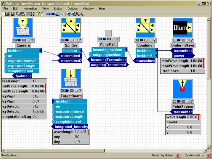
First, note that Splitter sends a copy of the complete incident wavetrain, i.e., light from both sources, to each sensor. However, because of the source and sensor wavelength parameter settings (highlighted by the red bars in the picture), the Camera only sees the PointSource, and the TargetBoard only sees the UniformWave.
If the wavelengths of the two sources were equal, and we still wanted to have each sensor see only one of the sources, then an extra distinguishing tag would have to be applied to each wave. WaveTrain provides "polarization" tags for this purpose.
Combining and separating light with polarization tags
At the end of the preceding example, we noted that Splitters and Combiners are not always enough to ensure that only the desired beams strike the desired sensors in a WaveTrain system. The WaveTrain machinery provides one additional degree of freedom for this purpose, namely the feature of "polarization" tags. "Polarization" is manipulated using library components like Polarizer and PolarizingSplitter. We put "polarization" in quotes here because WaveTrain's polarization has some unphysical aspects designed for convenience of simulation. For details on how to use the WaveTrain polarization tags, see the section on polarizers in the Modeling Details chapter.
Using Polarizers to separate light from different sources
At the end of the section on splitting and combining wavetrains, we mentioned that the additional feature of "polarization tags" was sometimes needed to achieve the system modeling goals. WaveTrain's polarization tags can represent some aspects of physical polarization, but the tags also have unphysical features. Their main purpose is really to assist in the combining and separating of beams within the WaveTrain interface restrictions, and not to provide a physically faithful representation of polarization phenomena.
A WaveTrain "polarization" tag (or polarization state) is
applied to an unpolarized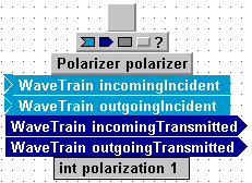 wavetrain by passing it through a
Polarizer component, whose interface is shown at right, and setting the
parameter polarization
to a positive integer. The unphysical aspects of the transmitted wave are
that
wavetrain by passing it through a
Polarizer component, whose interface is shown at right, and setting the
parameter polarization
to a positive integer. The unphysical aspects of the transmitted wave are
that
(a) the energy is the same as the incident, and
(b) any number of independent "polarization" tags (all positive integers) are
allowed.
Once a wavetrain is "polarized" in this manner, another Polarizer component can
later be used as an analyzer to pass or block a wavetrain depending on whether
the wave's state number is equal to or different from the
polarization tag of the
analyzer.
The polarization "analyzing" can be done with a combination of Splitters and Polarizers, but there is another WaveTrain library component that is frequently more compact for this purpose, namely the PolarizingSplitter. (In fact, by descending into PolarizingSplitter, we can see that it is a composite system that consists of a Splitter and two Polarizers). The use of PolarizingSplitter is illustrated in the example below.
All WaveTrain sources generate unpolarized light, unless there is some explicit statement to the contrary in the source documentation. Unpolarized light has a polarization state of 0. If we set the parameter polarization = 0 in a Polarizer component, that effectively deactivates it: any light, whether polarized or unpolarized, passes through it unchanged.
The following picture shows an example of how the polarization tags can be used. The two sources at the right of the picture have the same wavelength. We want to pass their light through the same atmosphere but then we want to sense the light from each source with a different sensor. Applying Polarizer tags immediately after the sources, and splitting the composite wavetrain later with a PolarizingSplitter allows the Camera to respond only to the PointSource, and the TargetBoard to respond only to the UniformWave. This system should be contrasted with the similar system picture in the introductory section on splitting and combining: in the latter case, polarization tags were unnecessary because the sources had different wavelengths and could be separated by using the wavelength sensitivity of the sensors. Remember that the system below could be extended to N sensors each receiving only one of N sources, because of the existence of an indefinite number of independent "polarization" tags.
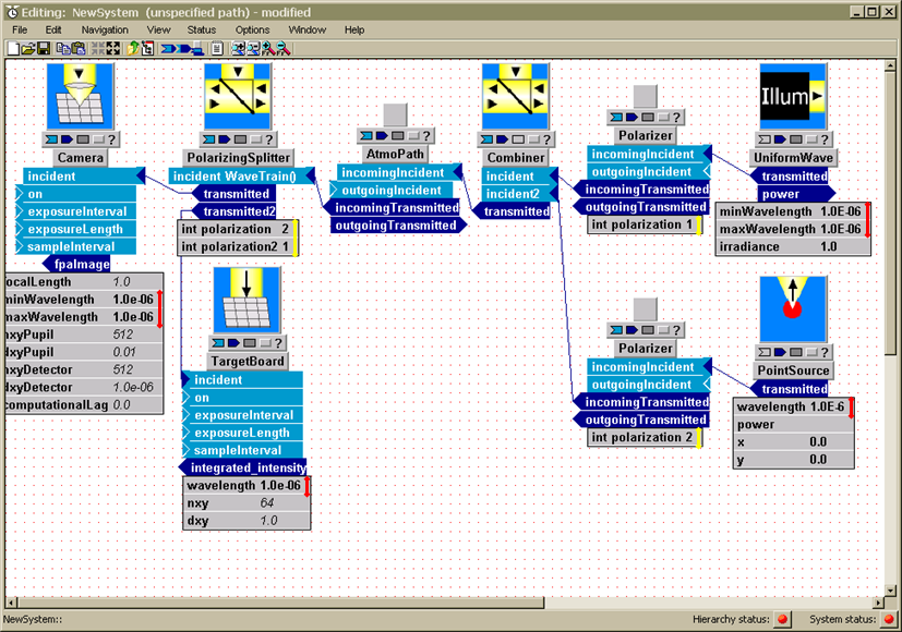
Eventually we plan to add physics-based modeling of polarization states to WaveTrain, but when we do we will still support the idealized model, because we have found the ability to separate light in this way to be very useful. For example in one case this made it possible to use the same light - and thus the same FFT propagations - to close the loop on multiple adaptive optics systems with different design parameters, then propagate scoring beams back from each, and separate them at the target. This greatly sped up execution, saving thousands of CPU hours in the course of a large parameter study.
Use of the Zernike function orthogonal basis set is common in optical
analysis. WaveTrain provides a number of components that facilitate the
creation of Zernike superpositions, decompositions and related manipulations.
Users should exercise caution in two respects when using these components:
(a) The WaveTrain components offer various normalization
and index ordering conventions (reflecting various usages in the general literature on
Zernikes).
(b) Zernikes as a mathematical basis set can of course be used to expand a
function f(x,y) of arbitrary physical units and significance. However, the
most common application is to expand a phase or OPD map, which is (or will later
be) associated with an optical phasor exp[i*f(x,y)]. In such cases, it is
usually important to be aware of whether the optical path length or difference (OPL or OPD)
is expected or provided in meters or in radians of phase.
In this section, we identify and discuss several of the key Zernike components, and we explain the index ordering, normalization and physical units conventions. WaveTrain's Zernike components are located in the ProcessingLib library that is accessible from the master library.
Browsing the ProcessingLib reveals a variety of components related to Zernike manipulations. The two basic operations are:
(1) To create a map f(xi,yj)
= Sk
ak*Zk(xi,yj) , from coefficients
ak and Zernike basis functions Zk, i.e., to create a superposition of Zernike basis
functions, use the component
ZernikeCompose.
Key inputs and parameters are the coefficient vector, ak, and
the (x,y) mesh specification. The output is a
Grid<float> variable that contains the f(xi,yj)
data. Notice that ZernikeCompose
does not directly create a wavetrain (i.e., a complex field) as output.
Typically (but not always), one would want to insert f(xi,yj)
as the phase map of a wave at some point in a WaveTrain propagation system.
The picture below shows a simple example, wherein Zernike phase aberrations are
added to a plane wave:
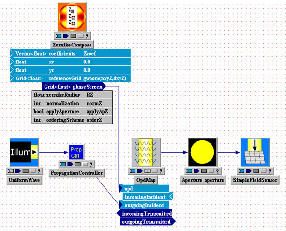
(2) To decompose a given function map f(xi,yj)
into its ak Zernike coefficients, use the component
ZernikeDecompose.
This function is the inverse of ZernikeCompose.
Notice that ZernikeDecompose
does not accept a wavetrain (i.e., a complex field) as input: the
input is simply the real function f(xi,yj) that is
to be decomposed.
Ordering conventions
WaveTrain's Zernike ordering and normalization options are described rather confusedly in the html help pages of the individual components. In the following two subsections, we attempt to clarify the key points.
Each Zernike basis function is a product of a radial and an angular function. As with other orthogonal expansions in 2D, the "natural" indexing to specify a particular basis function uses two indices. However, R.J. Noll wrote an influential paper applying Zernikes to atmospheric turbulence, and in this paper Noll introduced a mapping to a one-dimensional Zernike index. This type of 1D index is used to specify the input or output coefficient vectors, ak, in the Zernike components. A variation (still 1D) of the Noll ordering, used by Malacara, is also available in the WaveTrain components. Malacara's ordering differs from Noll's in the order of the azimuthal terms within each radial order.
Note that in the i/o of the basic routines, the
ZernikeCompose
input vector "coefficients"
ZernikeDecompose
output vector "ZernikeCoefs"
are ordered in the 1D convention of Noll or Malacara. Noll order is
specified by setting parameter "orderingScheme"=1,
and Malacara order is specified by setting "orderingScheme"=2.
The piston term (constant with respect to x,y) is omitted from all the basic WaveTrain Zernike components. The coefficients vectors start with tilt. The following picture shows image plots of WaveTrain's first 10 Zernike functions (Z1 to Z10) in the Noll ordering convention. Note that +x is vertically down in each subplot. Terms 1 and 2 are tilt, term 3 is quadratic focus, terms 4 and 5 are astigmatism, terms 6 and 7 are coma, terms 8 and 9 are triangular astigmatism, and term 10 is balanced spherical aberration and focus:
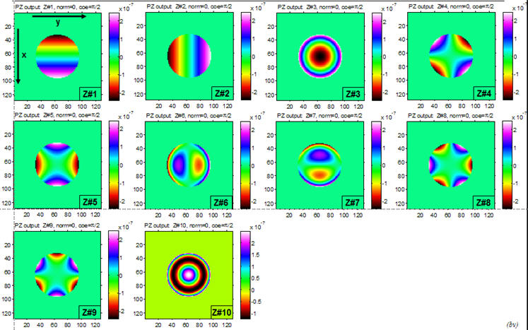
REFERENCES:
1)
Noll, Robert J., "Zernike Polynomials and Atmospheric Turbulence", J. Opt. Soc.
Am., Vol. 66, No. 3, pp. 207-211, 1976.
2) Malacara, D., and S.L. DeVore, "Interferogram evaluation and wavefront
fitting": pg. 465, Ch. 13 of Optical Shop Testing, 2nd.
ed., D. Malacara, ed., Wiley, 1992.
Normalization conventions
Several normalization conventions for the Zernikes may be found in the optical literature. The WaveTrain components all have a choice of normalization conventions, specified by the parameter "normalization". Two of the WaveTrain normalization choices are useful:
"normalization" = 0: The numerical value of each Zk(x,y) peaks at +1 at one or more points on the circle whose radius is the "Zernike radius".
"normalization" = 3: The rms deviation of each Zk(x,y), over the disk whose radius is the "Zernike radius", is equal to 1. Therefore, the numerical coefficient value ak will be the rms value of the product ak*Zk(x,y). Furthermore, in a sum of several terms, .f(xi,yj) = S(k=1,N) ak*Zk(xi,yj), the spatial variance of f will be the sum of the variances of the individual terms, i.e., var(f) = a12+...+aN2 . (This norm is called the "Noll/Malacara norm" in the component help pages).
Other values of "normalization" (which are described in the help pages for individual Zernike components) remain in the routines for historical reasons, but are not recommended.
The "Zernike radius"
The main significance of the "zernikeRadius" parameter has already been indicated in the preceding subsection on normalization conventions. In ZernikeCompose, the extra parameter "applyAperture" allows the generated Zernike terms to be set to zero or not, as desired, for (x,y) coordinates outside the "zernikeRadius".
Physical units
The mesh coordinates (xi,yj) and the Zernike radius, as with all lengths in WaveTrain, must be specified in meters. The Zk quantities themselves are unitless. Finally, the units in which ak, and thus f(xi,yj) = Sk ak*Zk(xi,yj), should be specified depend on how f(xi,yj) will be used by WaveTrain. A typical WaveTrain procedure would be to input f(xi,yj) into an OpdMap module, in order to apply f(xi,yj) as a phase perturbation on a passing wave (see the picture in Basic Zernike Components). In this case, since OPDmap interprets its input as an OPD in meters, the ak coefficients must be provided in meters. But of course a Zernike sum f(xi,yj) could be used in other ways, where f has different physical significance and different units..
Other Zernike components
The
ZernikeCompose/ZernikeDecompose routines explained in Basic Zernike Components should be considered the first choices in WaveTrain system construction requiring Zernike manipulations. However, in the course of WaveTrain development and application, a slightly different set of Zernike-related routines was also created. This alternate set of routines shares some but not all features and conventions of ZernikeCompose/ZernikeDecompose.The "PhaseZernikeXXX" component group:
The component
PhaseZernikeOPD
is conceptually equivalent to
ZernikeCompose.
That is, its principal purpose is to accept a set of input coefficients, and
then output the sum f(xi,yj)
= Sk
ak*Zk(xi,yj), on a specified
(xi,yj) mesh. The principal differences are:
(i) To produce an output f in meters,
PhaseZernikeOPD requires
input coefficients in radians of phase at a specified reference
wavelength. The output, in meters, is then appropriate for input into the
OpdMap module, exactly as was
done in the
ZernikeCompose illustration
in Basic Zernike
Components.
(ii)
PhaseZernikeOPD
requests a Zernike diameter (which is simply called "aperture diameter"),
whereas
ZernikeCompose requests a
Zernike radius.
(iii)
PhaseZernikeOPD has
parameters named "m_vec" and "l_vec" that allow extra selection freedom by
specifying that only certain subsets of the input coefficient vector elements be
used when composing the Zernike sum.
In other respects, the ordering and normalization convention options for the
coefficient input vector are identical in
PhaseZernikeOPD and
ZernikeCompose .
There are several other special-purpose Zernike-related components whose i/o conventions match PhaseZernikeOPD. The most important are PhaseZernikeDM, and PhaseZernikeSlopes:
PhaseZernikeDM takes an input vector of Zernike coefficients, internally composes the sum function f, and generates corresponding deformable-mirror (DM) commands which are organized as required for input into the WaveTrain DM component.
PhaseZernikeSlopes takes an input vector of Zernike coefficients, internally composes the sum function f, and generates the corresponding wavefront-sensor (WFS) slopes, corresponding to Shack-Hartmann subapertures whose geometry is specified according to the WaveTrain WFS procedures.
Adaptive optics models (wavefront sensors, deformable mirrors, tilt trackers)
In the present section of the User Guide, we discuss certain important features of the core WaveTrain library components needed for wavefront sensing and correction. These core components are HartmannWfsDft, DeformableMirror, and BeamSteeringMirror.
The generation of some of the geometric input specifications and the reconstruction matrices required by HartmannWfsDft and DeformableMirror is a complex task. A separate Adaptive Optics Configuration Guide has been written to explain the extensive WaveTrain tools provided for that purpose. We recommend that the user first study the present section of the general User Guide, and then dive into the Adaptive Optics Configuration Guide as needed.
Another way of getting started with adaptive optics (AO) modeling in WaveTrain is to use the BLAT example system provided in the WaveTrain examples directory (wavetrain\examples\BLAT01\). The BLAT acronym stands for Baseline Adaptive Optics and Tracking. BLAT is flexible enough so that users can implement a variety of scenarios by modifying just the provided runset, or by making minor modifications to the BLAT block diagram. BLAT may also help users to get started without diving into all the details of the Adaptive Optics Configuration Guide. In any case, users should read the present section for general orientation.
Wavefront Sensor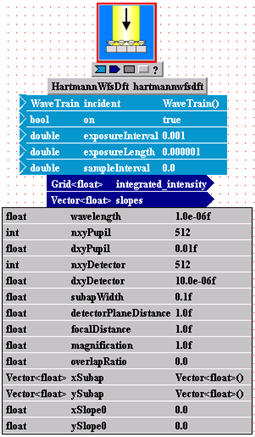 (Shack-Hartmann)
HartmannWfsDft is the fundamental wavefront sensor (WFS) module provided in the general WaveTrain distribution. This component models a Shack-Hartmann wavefront sensor. The lenslet perimeters are assumed to be square, and neighboring lenslets are assumed to have a 100% fill factor.
The picture at right shows the interface of
HartmannWfsDft. The
component inputs are like those of Camera,
and are typical of any WaveTrain time-integrating sensor. The component
outputs are:
(i) an integrated-intensity map of all
the subaperture spots, at specified sensor output times
(ii) a composite vector, containing noise-free, high-resolution x and y
slopes for all the subapertures.
The component parameters are discussed in more detail below. The meaning
and setting procedures for some of the parameters are far from intuitive, so this
section will be fairly lengthy.
CAUTION: by itself, HartmannWfsDft produces somewhat idealized results. In order to obtain the subaperture slopes as computed from specified WFS focal-plane-array pixel dimensions and noise characteristics, the HartmannWfsDft module must be followed by SensorNoise and HartmannWfsProcessing. A complete wavefront-sensing system based on subaperture centroids can be constructed using HartmannWfsDft alone, but that would be idealized to the extent that it would not account for sensor noise (finite light level) nor the pixelization error in computing spot position due to the finite focal-plane-array pixel size).
There are two separate setup steps required to enable the use of HartmannWfsDft. The first setup step is to specify a set of scalar parameters that define certain subaperture dimensions and computational controls on the subaperture spot patterns. The HartmannWfsDft parameters in question are the set subapWidth, focalDistance, detectorPlaneDistance, magnification, dxyDetector, overlapRatio, and nxyDetector. The setting rules are rather involved, and the procedure has a number of subtleties that require careful attention. This setup step is discussed in the following subsections.
The second setup step is the specification of the 2D layout of the subapertures. The 2D layout is summarized in two vectors that contain the x-coordinates and the y-coordinates of the subaperture centers. The tool provided to create these vectors is a graphical MATLAB helper program called AOGeom. Usage of this tool is explained in the Adaptive Optics Configuration Guide. The two coordinate vectors that are created and saved by AOGeom must be read into the HartmannWfsDft parameters xSubap and ySubap. The Adaptive Optics Configuration Guide illustrates the setting-expression syntax that can be used for that purpose.
WFS modeling in "object space" - general concepts
In WaveTrain modeling in general, and adaptive optics (AO) systems in particular, we frequently do not want to include the details of the actual optical train that leads from the physical primary aperture to the physical sensor plane. The actual optical path may contain numerous beam transport, compression and reimaging steps. For many purposes, there is no point in representing all of this step-by-step in WaveTrain. For many purposes, the diffraction and imaging steps between the primary aperture and the sensor plane can be represented in terms of an equivalent-lens/lenslet system, with equivalent focal length that acts in the primary entrance pupil, or in "object space". This is the same modeling principle discussed in a much earlier section of the User Guide.
When the "object-space" approach is applied to the modeling of a Camera subsystem, the key modeling requirement is that the focal-plane sensor pixels subtend the desired angle in object space. In this approach, the numerical values of the focal length and sensor pixel width specified in the Camera module are arbitrary, as long as their ratio is the correct object-space angle. Frequently, WaveTrain modelers assume a standard focal length of 1m for this purpose. Now, when modeling a Shack-Hartmann WFS, which is really a collection of side-by-side cameras, we usually use the same general principle of "object-space" modeling. However, in the case of the WFS, the simplest (without loss of generality) modeling approach involves an extra constraint on the equivalent focal length: in this case, the standard choice of 1m is not the best, because it introduces an extra complication which must be handled by means of the somewhat peculiar
magnification parameter that appears in the HartmannWfsDft parameter list. The following subsections contain a detailed explanation of the suggested parameter-setting procedures for HartmannWfsDft.WFS modeling - details of "Approach 1"
The mapping from a physical WFS to its object-space or entrance-pupil equivalent is shown by the mapping between Figure B and Figure A below:
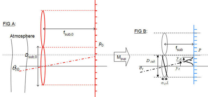
Figure B shows the physical WFS lenslets, whose parameters are Dsub, fsub. In the focal plane of the lenslets, we have a sensor pixel width p, where p is one pixel of a 2D array sensor. (In the physical system, there will probably be a subsequent reimaging of the p focal plane, in order to create a desired p value from a given array sensor whose physical pixel pitch is actually some other value p'; see Figure (MC1) in the later discussion for a concrete example). The equivalent lenslet system (Figure A) lies in the entrance-pupil plane of the actual optical system. The transverse magnification from A to B is the pupil magnification Mpup, a design parameter of the actual optical system. The parameters of the equivalent WFS system are indicated by "0" subscripts.
It is clear that Dsub should scale according to
Dsub,0 = Dsub
/ Mpup.
(Eq. 1)
In the Figure A-B mapping diagram, we also assume that p scales according to
p0 = p / Mpup
.
(Eq. 2)
(Equation 2 is a modeling choice, not a requirement. A
different choice could be made, but
Eq. 2 is the simplest choice; furthermore, there is no loss of generality
because of this choice).
Now as discussed above, a key constraint that we must observe in order to
create a faithful object-space model is the correct mapping of the angle
subtended by a sensor pixel (or more precisely, any field angle). In the
physical WFS, we have by definition
qsnspix = p / fsub ; similarly,
in the equivalent entrance-pupil system, we have
qsnspix,0 = p0 / fsub,0 .
On the other hand, from first-order optics, we know that any field angle (or we
can think in terms of a system chief ray) must map according to
qsnspix,0 =
qsnspix * Mpup
(Eq. 3)
Combining the last three formulas, we see that they require
fsub,0 = fsub
/ (Mpup)2
(Eq. 4)
In sum, we can create a consistent entrance-pupil model of the Shack-Hartmann WFS, as diagrammed in Figures A-B, if we satisfy the 4 conditions of Eq. (1-4). The first three may be consider "obvious" properties of transverse magnification, but the longitudinal magnification required by Eq. (4) is less obvious.
Defining the entrance-pupil system without a physical-system design:
In many simulation exercises, the physical dimensions
{Dsub, fsub,
p, Mpup}
(Spec "S1.1")
may not be known, because there is no actual optical system design yet. In
such cases, which are typical of generic AO system modeling, there are various
combinations that one could use to define the WFS system. One option is to
specify the set
{Dsub,0 ,
qsnspix,0 , p0}
(Spec "S1.2")
as the fundamental input specifications, with only the picture of Figure (A) in
mind.
Note 1: instead of p0 directly in "S1.2", the most meaningful
spec may be the "number of sensor pixels per subaperture", i.e., the ratio Npix_per_sub
= Dsub,0 / p0 .
Note 2: the Dsub,0 value would generally chosen on
the basis of an expected atmospheric Fried-r0 value.
Note 3:
qsnspix,0 is independent of Dsub,0 , but
there is the following constraint. Since the subaperture diffraction lobe
width is
The set "S1.2" in conjunction with Figure (A) is a complete and consistent specification, as proven by the preceding analysis. However, the HartmannWfsDft module requires a
focalLength specification, and this must be simply fsub,0 = p0 / qsnspix,0.Summary of HartmannWfsDft parameters thus far:
The preceding analysis has explained how to set the HartmannWfsDft parameters subapWidth and focalDistance. Usually, we also set detectorPlaneDistance = focalDistance. If one wants to study the effects of defocus on the WFS operation, one can set detectorPlaneDistance to a value of interest different from focalDistance.
Next, we discuss the HartmannWfsDft parameters dxyDetector, overlapRatio, and nxyDetector.
Fourier transform propagation control parameters in HartmannWfsDft
The parameters dxyDetector and overlapRatio control the numerical propagation mesh used by the Discrete Fourier Transform (DFT), when a given subaperture spot diffraction pattern is computed. Given the complex optical field incident on its lenslet plane (see Figure A). HartmannWfsDft first extracts that portion of the field incident on a given subapWidth, interpolates the incident field onto a desired (usually finer) mesh, pads that with a certain band of zeros, and finally performs a DFT to obtain the sensor-plane spot intensity pattern for the given subaperture. This operation is performed separately for each subaperture.
The two parameters dxyDetector and overlapRatio determine the DFT numerical mesh as follows. First, dxyDetector specifies the spacing of the mesh on which HartmannWfsDft will report its integrated_intensity output map. The numerical value dxyDetector should be selected so that the diffraction-limited spot is reasonably well sampled: this means at least two samples per (wavelength/subapWidth)*focalDistance.
The more mysterious parameter is
overlapRatio: this specifies
the total width of the computational mesh for a single subaperture spot pattern.
Physically, diffraction causes the spot pattern to have unlimited width; for
numerical computation one must decide where to cut this off.
overlapRatio specifies the
cutoff in terms of the subapWidth,
as follows: overlapRatio
= 0 means that the mesh on which the spot pattern is computed in the
sensor plane spans
exactly one subapWidth;
overlapRatio = 1 means
that the mesh spans out to one subaperture width on each side of the
saubaperture in question, etc; fractional
values are allowed. If overlapRatio
> 0 is specified,
HartmannWfsDft will eventually
add the overlapping intensity contributions in order to produce its net
integrated_intensity sensor-plane output
map.
(For a fixed dxyDetector, larger
values of overlapRatio of course
require longer numerical computation times. Given that some thresholding is usually applied later when computing the spot centroids,
overlapRatio = 0 is
often satisfactory).
Finally, parameter nxyDetector specifies the total width
of the mesh (in number of mesh points) on which
HartmannWfsDft produces the net integrated_intensity
output map. This should be specified large enough to contain all the
subapertures in the 2D layout. A typical setting would be
nxyDetector = (Dsub,0
/ dxyDetector) *
Nmax,sub + 1 ,
where Nmax,sub is the number of subapertures across the
maximal dimension of the 2D layout.
Remaining parameters of HartmannWfsDft
To complete the discussion of Approach 1 to setting WFS parameters, we now explain the remaining parameters.
magnification: In approach 1, the magnification parameter should be set to 1. This means it will have no effect on the computations. This modeling parameter is NOT the pupil magnification Mpup that played a prominent role in Figures A-B and the related discussion. magnification is only needed if we use Approach 2 to defining WFS parameters.
dxyPupil, nxyPupil: These parameters are only used if the "wavesharing" feature is invoked in Wavetrain propagations. "Wavesharing" is an advanced, not fully-debugged feature of WaveTrain. For most WaveTrain use, dxyPupil and nxyPupil should be set to dxyprop and nxyprop, respectively. (Unless "wavesharing" is invoked, the numerical values are actually never used).
xslope0, yslope0: These are the initial values of the slopes, prior to any sensor information being generated in the WaveTrain simulation. The values are usually set to 0.0.
slopes output: high-resolution and recomputed slopesHaving completed the discussion of Approach 1 to setting WFS parameters, we pause for a moment to discuss some features of the HartmannWfsDft outputs. After that, we return to the alternate approaches to specifying the WFS parameters.
integrated_intensity:
this is a composite integrated-intensity map of all the subaperture spots, at all the specified sensor output times. It is recorded on the spatial mesh {dxyDetector, nxyDetector}.slopes: this is a composite vector containing, first, the x-slopes (tilts) in each subaperture, followed by the y-slopes in each subaperture. The slopes are in units of radians. The order of subapertures within the vector is explained in detail in the Adaptive Optics Configuration Guide.
Each slope is determined from the centroid of the respective subaperture intensity pattern, as recorded on the dxyDetector mesh, with a 10% threshold applied before computing the centroid. The threshold is applied separately in each subaperture processing region. We refer to these slopes as the "high-resolution" slopes.
The "high-resolution"
slopes generated as discussed above are intended to be an idealized computation of
the subaperture tilts. To more accurately model the centroids computed
from an actual 2D array sensor placed in the lenslet focal plane, one should add
the WaveTrain components SensorNoise and
HartmannWfsProcessing.
SensorNoise would take as an input the
integrated_intensity
output of HartmannWfsDft. SensorNoise serves two functions:
(i) SensorNoise allows the spatial
integration of the high-resolution
integrated_intensity pattern into physical-pixel powers. The
"physical pixel" width is the p0 parameter discussed earlier.
Note that we used a mental picture of the desired p0 while defining
the
HartmannWfsDft parameters, but
the sample mesh in the sensor plane was actually the finer
WFS modeling - details of "Approach 2" (using magnification ≠ 1)
Approach 1 made a simple and physically clear modeling choice about the {p , p0} transverse scaling. In that approach, p/p0 is exactly the same as the pupil magnfication Dsub/Dsub0. The pictorial representation of the model is Figure A-B. As a consequence, we saw that the longitudinal ratio fsub / fsub,0 had to scale as the square of the pupil magnification. In Approach 1, The HartmannWfsDft parameter called magnification, which is NOT the pupil magnification, is set to 1 (i.e., the parameter is inactive).
A different approach is also possible. This alternate "Approach 2" has been used in a variety of WaveTrain applications, including the important example system BLAT. Approach 2 is somewhat more convoluted, and requires a peculiar "magnification" operation that is implemented by the HartmannWfsDft parameter called magnification.
Approach 2 is based on setting fsub,0 (focalDistance) equal to the arbitrary reference value 1 m. The motivation for the choice focalDistance = 1 was briefly reviewed in the introductory section on WFS modeling in object space. After this choice, Approach 2 completes the specifications by also choosing Dsub,0 and qsnspix,0 . A consistent model can be built on this basis, but it requires an extra adjustment. The problem is that the combination {fsub,0 = 1m, qsnspix,0 } contradicts the intuitive scaling choice p/p0 = Dsub/Dsub0. As we noted before, this is not wrong, but it requires an extra adjustment to the center-center separations of the subaperture regions in the sensor plane. This adjustment factor is what is generated by setting magnification ≠ 1. For an example of the actual setting expression assignments, we refer the user to the WaveTrain distribution's BLAT example system.
As a final comment on the use of
magnification
≠
1, we note the following peculiar property. The diffraction lobe of a
subaperture has the width
(wavelength/subapWidth) * focalDistance
= (wavelength/subapWidth) * (1m),
unaffected by
magnification
, but the center-center separation of the neighboring subaperture diffraction
patterns is the subaperture separation multiplied by
magnification.
In all of the above, we assumed that an adequate simulation model could be constructed without explicitly modeling the physical propagation through the optical train. (Or said more precisely, we assumed that an adequate simulation model could be constructed using just a single physical propagation from the equivalent lenslet plane to the equivalent focal plane.) This is certainly true in many cases. On the other hand, for a faithful model of certain complex systems, it may be necessary to model engineering details of the system by explicitly including beam compression stages and physical propagations between optical components. WaveTrain has components in the general distribution that allow this extra level of detail, if users feel that is necessary for their modeling purposes.
Miscellaneous comments
Lenslet Fresnel number in Approach 1:
Since Mpup = Dsub / Dsub,0 , Equation (4)
is equivalent to the statement
(Dsub,0)2
/ (l
fsub,0) = (Dsub)2 / (l
fsub) ,
in other words, Equation (4) is equivalent to saying that fsub,0 must
be chosen to conserve the Fresnel number of the lenslet system.
Explicit design of the reimaging stages:
For more complete visualization of the WFS parameter setting procedures, it may be helpful to consider a more complete optical design from primary aperture to physical WFS. Figure (MC1) shows such a layout.
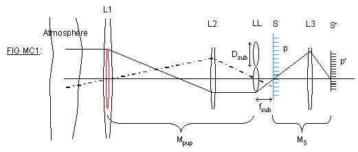
The first key operation in Figure (MC1) is reimaging of the primary aperture L1 onto the actual WFS lenslet plane LL. This occurs with a transverse magnification Mpup. Figure (MC1) shows this reimaging operation being done by a single focusing element L2. In general, the operation may be accomplished by multiple pupil relays, but it is always characterized by an overall Mpup. The red lenslet in the L1 plane is the geometrical back-image of a physical lenslet. In the focal plane S of the physical lenslets, we have the initial focal spots formed by the lenslets. In order to mate available lenslet hardware with available 2D-array sensor hardware, there may be a reimaging of the focal spots, as indicated by the MS magnification operation performed by L3. The symbol p' denotes the actual pixel width on the physical 2D-sensor plane, whereas p denotes the back-imaged size of the sensor pixels in the original lenslet focal plane S.
Concluding remarks
In the present section, we have reviewed procedures for setting the key scalar parameters in HartmannWfsDft. As noted previously, in order to complete the specification of the 2D layout of the WFS subapertures, use of the AOGeom tool is also required. The Adaptive Optics Configuration Guide explains how to use this tool to create subaperture 2D-layout data for input into the HartmannWfsDft parameters
xSubap and ySubap.Remember also that the example system and tutorial information for the BLAT model.provides a working WaveTrain AO system, which users can consult for further guidance or modify as they wish for their own purposes.
To use the information from a wavefront sensor to produce real-time correction of a wavefront, we require a deformable mirror (DM). The figure at right shows the interface of WaveTrain's DeformableMirror component. DeformableMirror applies specified mirror actuator commands to generate a shape deformation that corrects the wavefront incident on the DM. The commands fed to DeformableMirror must be generated by first multiplying the composite vector of Shack-Hartmann tilts by a "reconstructor" matrix. Then, one would apply a Gain factor and generate the new actuator commands for input to DeformableMirror.
As was the case with the WFS, use of
DeformableMirror in a
WaveTrain system requires a preliminary setup procedure. In this setup
procedure, we must
(i) specify certain geometric parameters of the DM actuator layout,
(ii) specify a DM influence function, and
(iii) generate.a reconstructor matrix (which will map measured WFS slopes into a
mirror shape correction.
The procedure starts by using the same AOGeom helper program
(MATLAB-based) that was used to define the 2D WFS layout. Then, a variety
of associated MATLAB tools and routines can be used to generate the
reconstructor matrix.
A separate Adaptive Optics Configuration Guide is provided to explain the details of the AOGeom and associated WaveTrain tools. We recommend that the user first study the present section of the general User Guide, and then dive into the Adaptive Optics Configuration Guide.
Finally, remember that the example system and tutorial information for the BLAT model provides a working WaveTrain AO system, which users can consult for further guidance or modify as they wish for their own purposes. BLAT may help users to get started without diving into all the details of the Adaptive Optics Configuration Guide.
In addition to a WFS and DM, many AO systems contain a tilt-tracker
subsystem. The purpose of the tilt tracker is to
(i) sense the average tilt of the wavefront, and then
(ii) compensate that tilt before presenting the residual perturbed wavefront to
the WFS-DM subsystem.
This typically allows the DM to operate with reduced actuator-stroke
requirements. In some cases, a tilt-tracker alone may comprise the
complete AO system.
The key new component that we need to perform tilt tracking in WaveTrain is
BeamSteeringMi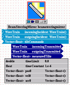 rror.
The figure at right shows the interface of WaveTrain's
BeamSteeringMirror component.
rror.
The figure at right shows the interface of WaveTrain's
BeamSteeringMirror component.
An average tilt can be sensed in various ways. The most basic would be to split off a portion of the wavefront into a Camera component, and then compute the centroid of the image (or some other measure of image "center"). Centroids can be computed, for example, by using the FpaProcessing module. Given the centroid angular position, one would apply a desired Gain factor and then generate a new tilt command for input to the BeamSteeringMirror module. The BeamSteeringMirror module then modifies the tilt of the incident wavefront before the wavefront passes on the WFS-AO subsystem and to system imaging cameras.
The centroid computation is only one way of determining the tilt correction to be applied. More complicated algorithms, such as correlation measures, may be more appropriate for certain situations. Such algorithms are not provided in the general WaveTrain distribution, and must be custom-coded. In all cases, though, the tilt compensation is carried out by a final tilt command fed to BeamSteeringMirror.
Again, the example system and tutorial information for the BLAT model provides a working WaveTrain AO system, which includes a centroid-based tilt tracker. Users can consult the BLAT system for further guidance, or modify it as they wish for their own purposes. BLAT may help users to get started without diving into all the setup details from scratch.
When modeling optical systems it is often necessary to model point sources. A point source can provide a direct measurement of a system's point spread function (PSF) and optical transfer function (OTF). For adaptive optics systems, a point source beacon maximizes the Strehl ratio. Off-axis point sources can be used to measure the effects of anisoplanatism. A single point source can be used to construct the image of a compact (i.e. smaller than an isoplanatic patch) incoherent source; multiple point sources can be used to construct the image of an extended incoherent source. Because of these special properties, point sources (actually "effective" point sources, such as a laser coming out the end of an optical fiber) are often used for calibration and experiments.
From the standpoint of theory - geometric optics or Rytov theory - point sources are easy to handle; for wave optics simulation this is not the case. In wave optics simulation a wavefront is modeled by a two-dimensional mesh of complex numbers. The mesh necessarily has both finite resolution, typically on the order of centimeters, and finite extent, typically on the order of meters. An ideal point source is infinitely compact, and radiates light uniformly in all directions; the outgoing wavefronts are complete spheres. Close to the source, the wavefront curvature goes to infinity. Far from the source, the wavefronts become far too large to represent on a practical mesh. This means that the direct approach - directly mapping the theoretical model to a numerical model - does not work.
The standard solution to this problem relies upon the fact that we are typically interested in only a small portion of the light from the source, the part that enters the aperture of the system of interest. One has to balance the desired characteristics for the field at the source plane with those at the aperture plane, taking into account the requirements of numerical propagation. At the source plane we simply want the field to be as compact - as pointlike -as possible. At the aperture plane, we want the field to have uniform amplitude over the aperture with a spherical phasefront centered on the source, because that is what we would expect for a true point source. When turbulence is present the instantaneous fields will be scintillated, but the time-averaged amplitude should still be uniform across the aperture. The time-averaged phase is ill defined, but the time-averaged phase gradient should correspond to a pure focus.
These requirements can be satisfied by constructing a field mesh at the aperture plane which has uniform amplitude, and the right phase curvature, over a region somewhat larger than the aperture, then doing a vacuum propagation back to the source plane. This is one of two methods supported by WaveTrain, and is the default. The second method emulates a technique that is often used by other analysts. This second technique is to start with a field at the source plane that has just a single nonzero mesh point, then apply a spatial filter which is unity over the angular region somewhat larger than the subtense of the aperture. This is essentially equivalent to the first method, except in the case where the nonzero region of the spatial filter chosen exceeds the subtense of the field mesh at the aperture. Ordinarily this would lead to problems due to wraparound, but these problems can be avoided by the judicious use of absorbing boundaries and spatial filters.
In the back-propagation method, the reason for making the uniform amplitude region larger than the aperture is to allow for scattering due to turbulence, as represented by the phase screens. For a true point source, the average amplitude is the same everywhere on a wavefront, and for any given point energy is as likely to be scattered in as scattered out. For our pseudo point source, points just inside the uniform amplitude region are more likely to lose energy then to gain it; this reduces the time-averaged amplitude for these points. By making the uniform amplitude region larger than the system aperture we can reduce or eliminate this effect for points inside the aperture. How much larger? That depends on the turbulence strength, the wavelength, the propagation geometry, and our error tolerance. As far as we know, no one has yet done a systematic study to look at this, although it would be straightforward.
If the uniform amplitude region at the aperture plane has a sharp edge, there will be significant energy at high spatial frequencies, which means that the field at the source plane will be less compact than we might like. If the uniform amplitude region is circular, the intensity at the source plane will be an Airy pattern, with its characteristic rings. By "softening" the edge of the uniform amplitude region, e.g. with a gaussian or cosine roll-off, we can reduce the high frequency content, resulting in a more compact field at the source plane. Unfortunately, this is not without cost. The roll-off region increases the size of the region of nonzero field, which is one of the factors that governs the minimum size of the mesh we can use, and simulation execution time increases roughly as the square of the mesh size.
We did a series of experiments in Matlab to compare the effects of different roll-offs. We used three different shapes: a gaussian truncated at two standard deviations, a gaussian truncated at three standard deviations, and a half cosine wave. We used a 256x256 mesh; with a circular region of unit amplitude 64 mesh points across, and varied the width of the roll-off region from 1 to 32 meshpoints. Of the three shapes, we found that the two sigma gaussian was generally superior, in the sense that for a wide range of tolerances and roll-off widths, the maximum radius exceeding the tolerance was smallest for that shape. As an example, the figure below shows the field amplitude as a function of distance from the origin in mesh points for the three roll-off shapes. The amplitude for the two sigma gaussian is shown in blue, the three sigma gaussian is green, and the half cosine is red. For larger tolerances, greater than about .1 times the on-axis value in amplitude, or .01 in intensity, no roll-off helped. For very small tolerances, less than about .004 in amplitude, .000016 in intensity, the two sigma gaussian truncated was inferior to the other two shapes, owing to the high frequency content associated with the truncation, but we cannot think of any practical reason we would need to consider tolerances that small.
As one increases the width of the roll-off region, the maximum radius for a given tolerance tends to decrease in discrete steps, jumping from one Airy ring to the next smaller one. This effect is shown in the first figure below, where we used a tolerance of .01 in amplitude (equivalent to .0001 in intensity) and the two sigma gaussian roll-off shape. For a given size mesh, there is a tradeoff between the radius of the uniform amplitude region and the width of the roll-off region, because the sum of the two must be less than one fourth the width of the mesh. If we hold the sum of the two constant, while varying the ratio between them, we find that the width of the source pattern generally decreases as we increase the width of the roll-off region, but there are local minima, related to the discrete steps we saw before - see the second figure below. This suggests that it would behoove one to always choose a roll-off width corresponding to one of the minima, but that holds true only if there is some special significance about the tolerance chosen. If we change the tolerance, the minima shift. This raises the question of what tolerance we should use, or to put it another way, what field amplitude, as a fraction of the maximum, do we consider "negligible"? This depends upon the application. If we wish to model something like the ABLE ACE Differential Phase Experiment, which measured the differences between the fields received from two closely space point sources, we will need to be very careful, especially in the low turbulence limit. For all other applications, we suspect it is a minor issue.
Discrete transitions in source field radius as the width of the roll-off region is varied while the width of the region of uniform amplitude is held constant.
Local minima in the source field radius as the width of the roll-off region is varied while the total width of the region of nonzero field at the aperture plane is held constant.
This brings me to my recommendations:
Use the default method (back-propagation). In the PropagationController, the parameter "pointSourceModel" should be set to "DEFAULT_PSM".
Following the guidelines in choosing parameter settings for modeling optical propagation, determine the mesh spacing and mesh dimension you wish to use. (for ABL ACT, a good choice is dxy=.02 and nxy=256. For ABL, try nx =512, and dx >= sqrt(2*lamda*z / nxy), where z is the range.)
Pick a "super-aperture radius" - the radius for the uniform amplitude region - a "fair amount" larger than the system aperture. (At some point we should do a study determine how large this should be, as a function of the propagation scenario).
If the minimum acceptable super-aperture radius is bigger than half the mesh width, you need a bigger mesh. You could increase the mesh spacing, but if that would make it too coarse to capture the turbulence effects you will have to increase the mesh dimension.
The super-aperture radius should now be less than or equal to half the width of the mesh. If there is any margin, you can use it in two ways: increase the super-aperture radius, and/or create a roll-off region. In some cases the overall size of the mesh will be driven by sampling requirements, rather than the size of the super-aperture, so you may find that you have plenty of room for both. In such a case, we recommend you make the super-aperture radius 15% of the mesh width, and the roll-off region 10% of the mesh width. The roll-off shape will be the two-sigma gaussian, so sigma would be 5% of the mesh width. When space is tighter, reduce or eliminate the roll-off region.
To implement these decisions, you will need to use a PropagationController, the WaveTrain component that controls all parameters related to optical propagation. Propagation Controller has a total of ten parameters but just three of these are used to control point source modeling: pointSourceModel, superApertureRadius, and edgeSigma. pointSourceModel should be set to "DEFAULT_PSM". superApertureRadius defines the radius of the uniform amplitude region. edgeSigma controls the width of the gaussian roll-off region. 2*superApertureRadius + 4*edgeSigma should be less than half the width of the mesh. edgeSigma and superApertureRadius are also used in modeling optical "speckle", seen when coherent light illuminates an optically rough surface; see how speckle is modeled. The same considerations apply in both applications, so it is appropriate to use the same values of edgeSigma and superApertureRadius for both point source modeling and speckle modeling.
If you wish to use the other method WaveTrain supports for modeling point sources, where the initial field at the source plane has just a single nonzero mesh point, set the parameter pointSourceModel to "MESH_POINT_PSM". Depending on the propagation parameters, you may also need or want to use spatial filtering and/or absorbing boundaries, as described in how to use spatial filters and absorbing boundaries. In this case, the parameters superApertureRadius and edgeSigma are ignored for point source modeling, but they may still be used in modeling speckle, if there is any, depending on the speckle model chosen.
Other methods are sometimes used for modeling point sources. Some analysts create a field at the aperture plane whose amplitude is a "supergaussian", and then back-propagate that in vaccum to the source plane. Other analysts use a large gaussian at the aperture plane, which maps to a small gaussian at the source plane. Both of these methods are reasonable, but have the disadvantage that the expected value of the received amplitude at the aperture will vary somewhat as a function of the radial distance from the origin. WaveTrain does not presently support the supergaussian technique, but it can be reasonably well approximated by choosing of superApDiameter and edgeSigma appropriately. WaveTrain does support the use of pure Gaussians - simply set superApDiameter to zero, and use edgeSigma to control the size of the Gaussian.
Optically-rough reflectors, and modeling of speckle
The WaveTrain library contains three basic rough-reflector modules. These are CoherentTarget, IncoherentReflector, or PartiallyCoherentReflector. By "rough reflector" we mean optically-rough in the sense that surface micro-roughness is large compared to one wavelength. We use the term "reflection" in a generic sense here: the modules could also be used to model an equivalent transmissive system, such as a ground-glass plate. In addition to the basic three systems, there are additional library systems built from these three, such as IncoherentDisk, CoherentRectangle, and IncoherentSource: these additional systems constitute various special cases or slight elaborations of the basic three. As implied by the names of the latter systems, the rough-"reflector" modules could also be used to model extended sources of various kinds, where the reflection of incident light is simply a simulation trick for modeling emission in the physical system.
The Wavetrain components named above make reference to various coherence states (coherent, incoherent, partially coherent). This signifies that the rough-reflector modules include features that simulate, with varying degrees of fidelity, the effect of non-zero optical bandwidths. We should emphasize that the use of these features is not the only way to model non-zero optical bandwidth in WaveTrain: an overview of methods is given elsewhere in the User Guide.
The rough-reflector modules can be found in the sub-library of the core WtLib called SourceLib. The reason for this association with sources is that, at the WaveTrain code level, the rough reflectors are implemented as a combination of a WaveTrain sensor and a WaveTrain source that generates the reflected (scattered) wave.
The physical models used in all the rough-reflector modules treat the optically-rough limit, i.e., surface micro-roughness large compared to one wavelength. The difference between the three fundamental modules is that they apply to different levels of temporal coherence of the incident light. CoherentTarget applies to the case where the coherence length of the illumination is long compared to the macro-depth of the target. This is the typical textbook laser-speckle case. IncoherentReflector is a relatively crude extension of the CoherentTarget concept that attempts to treat the limit where coherence length of the illumination is short compared to the macro-depth of the target. PartiallyCoherentReflector is a more physically-based model than IncoherentReflector, and carefully treats the intermediate case where coherence length of the illumination is of the same order as the macro-depth of the target. The key additional phenomenon that we model using IncoherentReflector and PartiallyCoherentReflector is the reduction in speckle contrast due to the finite temporal coherence of the illumination.
Recently, WaveTrain has introduced a fourth fundamental type of rough-reflector or extended source modeling approach, called Light Tunneling. The usage does not exactly parallel the other rough-reflector modules, because the Light-Tunneling modules work together only with special sensor modules.
CoherentTarget
Basics
CoherentTarget is the simplest of the three basic modules. CoherentTarget applies to the case where the coherence length of the illumination is long compared to the macro-depth of the target. This is the fundamental laser-speckle case treated in every modern-optics textbook.
When an optically rough surface is illuminated by a monochromatic beam, the phase differences across a surface of the exiting wave are still constant in time, although the phasefront becomes extremely rough. The assumption used in the basic theoretical treatment is that, in an exit plane after reflection, the phase of the exiting beam is uncorrelated from point to point, and has a standard deviation much greater than 1 wave (or equivalently, the mod-2
p phase is practically uniformly distributed over 2p radians). In accordance with this concept, CoherentTarget works by initially defining a spatially uncorrelated exit phase map, and propagating the resulting beam though the remainder of the WaveTrain system. In addition to internally generating the random-phase map, f(x,y), CoherentTarget allows the user to specify an intensity reflectance map, R(x,y), where (x,y) is transverse to the nominal propagation direction. R(x,y) allows the user to specify a target of arbitrary shape and non-uniform reflectance strength across the target. .Some details
In the real world, the roughness of the phasefront causes the reflected light to be scattered over a very broad angular range. Treating this in simulation involves some subtleties. As in the case of a point source, it is not possible to model the entire speckle wavefront, but neither is it necessary. We are generally only interested in that part of the light that might eventually enter the aperture of the optical system in question, and so we can use techniques similar to those we use in modeling point sources. To be specific, the default speckle modeling approach is to begin by generating a wavefront where the amplitude is computed from the amplitude of the incident wavefront, the intensity-reflectance map of the rough reflector, and a phase that is spatially uncorrelated and uniformly distributed on (-p to p). We then perform a vacuum propagation to the aperture plane, and multiply the field by a weighting function of unity over a circular region somewhat larger than the aperture, then dropping smoothly to zero. Finally, we do a second vacuum propagation back to the source plane, which yields the initial speckle field we will use to propagate back through turbulence.
The net effect of this technique is similar to spatial filtering, smoothing the speckle phasefront enough to limit the angular spread of the light, but our approach offers a useful advantage: regardless of the size and shape of the incoherent reflector, from each point on the reflector we capture all the light headed toward the system aperture, and only that light, automatically. Using spatial filtering, light from every point on the reflector leaves with the same angular spread, and it is incumbent on the user to ensure that the spread is great enough that the light from every point fully illuminates the aperture. This creates an opportunity for error, and for large reflectors it can make it necessary to use larger propagation meshes than would otherwise be needed, because of the larger angular spread required to ensure full illumination of the aperture.
To specify speckle modeling parameters, you will need to use a PropagationController, as described in choosing parameter settings for modeling optical propagation. To use the default modeling approach, set the parameter speckleModel to DEFAULT_SM, as shown, and use superApDiameter and edgeSigma to specify the aperture plane weighting function; see the recommendations given in how point sources are modeled.
To use the more conventional approach of starting with a delta-correlated speckle field, then using spatial filtering, set speckleModel to DELTA_CORRELATED_SM, and then specify the spatial filter as described in how to use spatial filters and absorbing boundaries.
IncoherentReflector
Suppose we illuminate an optically rough surface with light whose temporal coherence length is short relative to the macro-depth of the target surface. By macro-depth we mean the changing distance between target surface and receiver, due to target surface tilt or 3D shape. In this situation, when the distance differences between a receiver-plane point and different target points exceed the light's coherence length, optical interference will no longer be possible at typical detector response times. Therefore, the contrast of the speckle pattern can be greatly reduced.
The
IncoherentReflector module
is a relatively crude attempt to model reduction in rough-surface speckle
contrast, while still allowing the propagated light to be influenced by
turbulence and other factors along the propagation path.
IncoherentReflector causes
the following calculations:
(i) generation of "nWaves" independent rough-surface phase
realizations, each on the principles of CoherentReflector (the value nWaves is
user-specified)
(ii) propagation of each of the nWaves reflected waves through the
remainder of the WaveTrain system
(iii) averaging at any sensor of the nWaves speckle irradiance patterns.
Note that the nWaves parameter is the only degree of freedom in the model (as
far as the partial coherence aspect is concerned).
As was the case in CoherentTarget, the IncoherentReflector allows the user to specify an intensity reflectance map, R(x,y), where (x,y) is transverse to the nominal propagation direction. R(x,y) allows the user to specify a target of arbitrary shape and non-uniform reflectance strength across the target.
The conceptual weakness of the IncoherentReflector model is that there is no general quantitative formula that accurately relates the simple nWaves parameter to the speckle reduction details that correspond to a general illumination scenario.
PartiallyCoherentReflector
In contrast to
IncoherentReflector, the
PartiallyCoherentReflector model contains a much more precise mathematical
model of the interaction between light of specified temporal coherence and a rough reflector with specified macro-depth. As in the simpler rough
reflectors, the model still generates a spatially-uncorrelated phase associated
with the surface roughness h(x,y). However, a user-specified
macro-depth profile, D(x,y), is also entered into the model, along with a
numerical value of the illumination temporal coherence length,
lc. WaveTrain begins by generating
nWaves
statistical realizations of a slowly-varying envelope (SVE) phasor consistent
with
lc. For a given SVE realization, a
reflected exit wave in the reference plane is formed from the incident complex
field in the reference plane by folding in the geometric OPDs corresponding to
h as well as D. After this, the exit complex field is
propagated by the usual WaveTrain means through the remainder of the Wavetrain
system. This sequence is carried out for each of the nWaves statistical
realizations of the SVE phasor, and at any sensor the resulting nWaves
irradiance maps are averaged. This full sequence of operations explicitly
represents the averaging reported by any square-law detector over the response
time of the detector (assumed long compared to the coherence time of the
radiation). The main "loose end" in the model is the number nWaves
required to achieve a reliable estimate of the average.
rough reflector with specified macro-depth. As in the simpler rough
reflectors, the model still generates a spatially-uncorrelated phase associated
with the surface roughness h(x,y). However, a user-specified
macro-depth profile, D(x,y), is also entered into the model, along with a
numerical value of the illumination temporal coherence length,
lc. WaveTrain begins by generating
nWaves
statistical realizations of a slowly-varying envelope (SVE) phasor consistent
with
lc. For a given SVE realization, a
reflected exit wave in the reference plane is formed from the incident complex
field in the reference plane by folding in the geometric OPDs corresponding to
h as well as D. After this, the exit complex field is
propagated by the usual WaveTrain means through the remainder of the Wavetrain
system. This sequence is carried out for each of the nWaves statistical
realizations of the SVE phasor, and at any sensor the resulting nWaves
irradiance maps are averaged. This full sequence of operations explicitly
represents the averaging reported by any square-law detector over the response
time of the detector (assumed long compared to the coherence time of the
radiation). The main "loose end" in the model is the number nWaves
required to achieve a reliable estimate of the average.
Users who wish a more detailed discussion of the PartiallyCoherentReflector model and input parameters, along with a validation study that compares numerical performance with a theoretical result, should consult an auxiliary document.
Light Tunneling
The Light Tunneling method is based on (i) explicitly representing a rough reflector by a mesh of point sources, which are propagated individually, (ii) introducing special interpolation methods to allow a relatively sparse mesh of points to be physically propagated, and (iii) at a sensor, adding irradiances due to the point sources. Because of features (i) and (iii), there is no rough-surface speckle at all when using this model: therefore, it is particularly appropriate for modeling fairly broad-band illumination. For a detailed discussion of the Light Tunneling method, see the auxiliary document LightTunnelMethodInWaveTrain.doc. The document describes the physical basis of the simulation method, describes the WaveTrain modules that implement the method, and shows a sample WaveTrain system and results.
WaveTrain components for data-type conversion
Occasions arise in WaveTrain model assembly where it
seems physically logical to connect one component's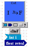 output to another component's input, but the data
types of the output and input have unfortunately been defined differently.
This could be as simple, e.g., as the output being single precision (type "float"),
and the input being double precision ("double").
Another example that may crop up is integer ("int")
versus boolean ("bool"). Conversions such
as these can be done using components from WaveTrain's
ConvertLib library, inserted
into the WaveTrain system in the System Editor. The figure at right shows
an example of such a component, named
output to another component's input, but the data
types of the output and input have unfortunately been defined differently.
This could be as simple, e.g., as the output being single precision (type "float"),
and the input being double precision ("double").
Another example that may crop up is integer ("int")
versus boolean ("bool"). Conversions such
as these can be done using components from WaveTrain's
ConvertLib library, inserted
into the WaveTrain system in the System Editor. The figure at right shows
an example of such a component, named
There is one other special type-conversion requirement that sometimes occurs in WaveTrain model assembly. This is the conversion of a "
float" to a "recallableFloat". This is accomplished with a special function syntax in a setting expression, as opposed to the insertion of a conversion component.How to use spatial filters and absorbing boundaries
In the wave optics modeling paradigm, on which WaveTrain is based, optical wavefronts are modeled using two-dimensional complex grids, and modeling optical propagation involves performing Fast Fourier transforms (FFTs) and applying quadratic phase factors to those meshes. This gives rise to a number of requirements related to the properties of the FFT, proper sampling of both the wavefront and the quadratic phase factors, most of which are discussed in how to choose parameter settings for modeling optical propagation. One of the most basic requirements relates to the fact that the meshes are necessarily very limited in extent, and while some of the light sources we wish to model are collimated, such as lasers, others are not, such as point sources, and the reflected return from an optically rough surface. These cases require special modeling techniques, and some of these techniques involve the use of spatial filters and/or absorbing boundaries; the purpose of this section is to explain how this can be done in WaveTrain. However the default techniques used by WaveTrain (see how point sources are modeled and how speckle is modeled) do not require the use of spatial filters or absorbing boundaries, so if you intend to use the default techniques you can skip this section.
The main reason you might wish to use spatial filters and/or absorbing boundaries is that under some circumstances it may allow you to use a smaller propagation mesh than would otherwise be required, and this can translate into a very substantial reduction in execution time. A spatial filter is a multiplicative weighting function applied in the spatial frequency domain; an absorbing boundary is a multiplicative weighting function applied in the spatial frequency domain. Applying spatial filter limits the angular spread of the light from all points on the mesh; applying an absorbing boundary removes light that approaches the boundary of the mesh. In each case the point is to ensure that no light reaches the edge of the mesh, because if it did, it would then reappear on the other side of the mesh, because of the periodicity of the FFT, leading to erroneous results. However you must take care to ensure that the use of filters and absorbing boundaries does not itself introduce errors, and in that we can offer little guidance, except to compare your results with those obtained without using either, but using a more conservative mesh. That said, some of the most experienced and respected experts in wave optics find spatial filters and absorbing boundaries to be invaluable tools.
WaveTrain allows you to specify one set of spatial filters and absorbing boundaries to be used for modeling the light from every light source in your system model, or to specify different filters and boundaries for specific sources. In both cases this is done using one or more Propagation Controllers, as described in how to choose parameter settings for modeling optical propagation. Three parameters of PropagationController are used:
oneTimeSpatialFilter (specifies a spatial filter to be applied on the first propagation step)
spatialFilter (specifies a spatial filter to be applied on each propagation step)
absorbingBoundary (specifies an absorbing boundary to be applied on each propagation step)
Note that each of these parameters has the same default value, "NullFilter()"; this means that by default no spatial filter or absorbing boundary will be applied.
Note also that each of these parameters are of the same data type, "const Filter&". That syntax will probably look a bit odd to those not familiar to C++, but it serves a useful purpose: it makes it very easy to add new types of filters, in case those we already support do not meet your requirements. At present, WaveTrain supports three types of Filters:
| Filter Type | Description |
| NullFilter() | No filter is applied. |
| RaisedCosineFilter(float ratio_flat) | Applies a 2-D "raised cosine" filter, which is unity in the central region (square or rectangular) and falls smoothly to zero at the edges, following a cosine curve through half a cycle. The size of the flat region relative to the size of the mesh is controlled by the constructor parameter ratio_flat. The cosine regions on each side extend from the edge of the flat region to the edge of the mesh. |
| LinkRaisedCosineFilter(float ratio_nonzero) | Applies a 2-D "raised cosine" filter, which is unity in the central region (square or rectangular) and falls smoothly to zero at the edges, following a cosine curve through half a cycle. The size of the flat region relative to the size of the mesh is controlled by the constructor parameter ratio_nonzero, and is equal to ratio_nonzero - 0.1. The cosine regions on each side extend from the edge of the flat region for five percent of the width of the mesh, so that the total width of the nonzero region is equal to ratio_nonzero times the width of the mesh: (ratio_nonzero-0.1+2*0.05). (Named for Don Link, of SAIC) |
Note that both of the non-null filters are defined relative to the size of the propagation mesh. In the case of an absorbing boundary this is just the spatial extent of the mesh in meters, equal to the product of the mesh spacing and the mesh dimension. Thus applying an absorbing boundary defined by the expression "LinkRaisedCosineFilter(0.9)" to a 256x256 mesh with a 2cm spacing, a total of 5.12m across, would result in a 4.096 m central region with unity transmission, surrounded on all sides by a 0.256 boundary where transmission falls from unity to zero, then another 0.256 boundary with zero transmission, extending to the edge of the mesh. Spatial filters, on the other hand, are applied in the spatial frequency domain, after a Fast Fourier Transform (FFT) has been applied to the propagation mesh. In the spatial frequency domin, each point on the mesh corresponds to a different propagation direction, where the largest spatial frequencies correspond to the widest propagation angles. The extreme propagation angles are given by +/- .5l/dxy, where l is the wavelength of the light and dxy is the mesh spacing. Thus applying a spatial filter defined by the same expression as above and to the same mesh as before, but in the spatial frequency domain, would result in unity transmission over an angular region bounded by +/- 4l/dxy, surrounded on all sides by a 0.05l/dxy region where transmission drops gradually to zero, and another 0.05l/dxy region with zero transmission.
At one point we anchored WaveTrain to ACS, another wave optics modeling code, for a case that involved the use of both spatial filters and absorbing boundaries, as specified by Don Link, the author of the other code. The scenario parameters were as follows:
|
Aperture Diameter, D |
52 cm |
|
Wavelength |
532 nm |
|
Range, z |
58.2 km |
|
Beacon Separation |
8 and 31 cm |
|
Turbulence Strength |
0.2, 1.0, and 5.0 x 10⁻¹⁷. No inner or outer scale. |
|
Phase Screens |
15 512x256 screens, grid spacing, dxy = D/70, no low order mode correction. |
|
Propagation: |
256x256 grids in ACS, 512x256 in WaveTrain, grid spacing = D/70. Collimated wave optics propagation (planar reference wave). Filters applied in both spatial and spatial frequency domains. (for details, see discussion below) |
|
Extended Source Modeling: |
Uniformly illuminated 50 cm disk, radiating 1 W/sr/m2 on axis. 16 random speckle realizations, different for each atmospheric realization. |
In the initial propagation, from the beacon to the first phase screen, a frequency domain filter was applied to limit the angular spread of the field. The exact form of the filter was a "raised cosine", unity in the center, zero at the edges, with a half cosine wave as transition. The full width of the nonzero region, expressed as an angle, was 1.5*nxy*dxy / z, while the width of the cosine transition regions on either side were 0.05*nx*dq, where dq = l / (nxy*dxy). After completing the propagation, a spatial domain filter, also a raised cosine, was applied. In this case, the full width of the nonzero region was 0.9*nxy*dxy, while the transition regions were .05*nxy*dxy. On the second and subsequent propagations a different frequency domain filter was used, where the width of the transition regions was unchanged, while the width of the nonzero region was 0.95*nx*dq. The same spatial domain filter was used in each propagation.
To implement this in WaveTrain, we used a PropagationController with the parameters spatialFilter and absorbingBoundary set to "LinkRaisedCosineFilter(0.9)" and "LinkRaisedCosineFilter(0.95)", respectively, and setting oneTimeSpatialFilter to "LinkRaisedCosineFilter(0.6844)". The last setting was obtained by dividing the width of the desired nonzero region by the size of the angular region corresponding to the FFT of the propagation mesh, taking into account the fact that each spatial frequency is related to a specific propagation angle by the wavelength: ratio_nonzero = (1.5*nxy*dxy / z) / (l/dxy) = 0.6844. Also, we used non-default techniques for modeling both point sources and speckle, designated by "MESH_POINT_PSM" and "DELTA_CORRELATED_SM", respectively, as described in how point sources are modeled and how speckle is modeled; both these techniques are designed to be used in combination with spatial filters and absorbing boundaries. Neither technique makes use of the parameters superApDiameter or edgeSigma, so we can set both to zero.
For the particular case we used in anchoring, the above choice of filters and absorbing boundaries seemed to work well, and allowed us to use a smaller propagation mesh than otherwise would have been necessary. Unfortunately, we cannot at this time offer general recommendations about what types of filters and absorbing boundaries will work for different propagation scenarios, and how that would affect the choice of other propagation parameters, such as the mesh size and spacing.
Using WaveHolder to avoid performing redundant propagations
Under certain circumstances it is useful to look at the performance of an optical system when the illumination entering the system is held constant; this effectively removes the effects of finite controls bandwidth, and can therefore help one to characterize the fundamental performance limits of the particular sensing and compensation scheme. For example, the optimum performance, in terms of Strehl, for a given adaptive optics system and given turbulence conditions can generally be obtained by closing the loop on a point source, holding both the platform and the target fixed, and setting the wind velocity to zero, so that outside of the optical system itself nothing is changing. Because the illumination reaching the system is unchanging in such cases, there is no reason to perform the FFT propagations used to compute the illumination more than once, but that is what would happen, unless you take special care to prevent it. This is done by inserting a special component, called WaveHolder anywhere along the common path of all the sensors looking at that illumination, prior to any active elements, such as a steering mirror or a deformable mirror, that would act on the illumination. Then, the first time the sensors try to look at the light incident upon them, the request will work its way all the way back to the point source, and propagations will be performed as usual. But after that, for the rest of the simulation run, WaveHolder will keep sending exactly the same light, and no further propagations will be performed. WaveHolder has three parameters, min_wavelength, max_wavelength, and polarization, which can be used to make it act only on part of the light that reaches it: Only light with wavelengths between min_wavelength and max_wavelength will be held, and if polarization is set to any value other than zero, only light with that same polarization state will be held. (see using Polarizers to separate light from different sources)
CAUTION: Be careful never to use WaveHolder when the incident illumination is changing; this will cause your simulation results to be wrong, and it may not be obvious. This is an easy mistake to make, because it is a common practice to first look at static cases, where the use of WaveHolder would be appropriate, and then to switch to dynamic cases, where would not be.
Data entry in subsystem parameters and inputs, and in the Run Set Editor
At this point we assume that the user has worked through some of the basic demonstration and tutorial material that introduced the procedures for assembling and saving a WaveTrain system, and for creating a run set for the system. (We refer specifically to the earlier Guide sections on assembling systems and the tutorial documents.) The present section reviews in a compact manner all the key features of System Editor and Run Set Editor (TRE) usage, and provides many details of data entry rules and syntax. (Note that the System Editor may alternatively be called the Block Diagram Editor in some documentation).
The user supplies input values to a WaveTrain simulation
in two different Editor windows:
(1) In the System Editor, the user must enter numerical values, symbolic
names, or expressions into "parameter" and sometimes "input" entry fields in
WaveTrain modules (subsystems).
(2) In the Run Set Editor (TRE), the user must assign values to the top-level
"System Parameters", and may create and assign values to "Run Variables".
The Run Variables comprise the simulation stop time, looping parameters, and
potentially other user-defined variables.
The following two figures illustrate a matching pair of System Editor and Run Set Editor (TRE) windows. In the present Guide chapter, we discuss in detail the syntax examples in these two figures, as well as many other important syntax rules for data entry.
The figure immediately below shows the System Editor
window for a simple WaveTrain system. First, note that all the information
bars attached to the subsystem icons have been pulled down. To accomplish
this we:
(1) Left-click the toolbar button indicated by the curved red arrow
(2) In the box that appears, left-click all the icons in the first column
(3) Finally, left-click all the "t", "n" and "v" icons to display all the Type,
Name and Value fields.
Note that "Inputs" (items in light blue background) have Type, Name and Value
fields. "Outputs" (items in dark blue background) have Type and Name but
no Value fields. Finally, "Parameters" (items in light grey background)
have Type, Name and Value fields. Type (i.e., data type) appears in the
first (leftmost) column, Name appears in the second column, and Value is in the
third column.
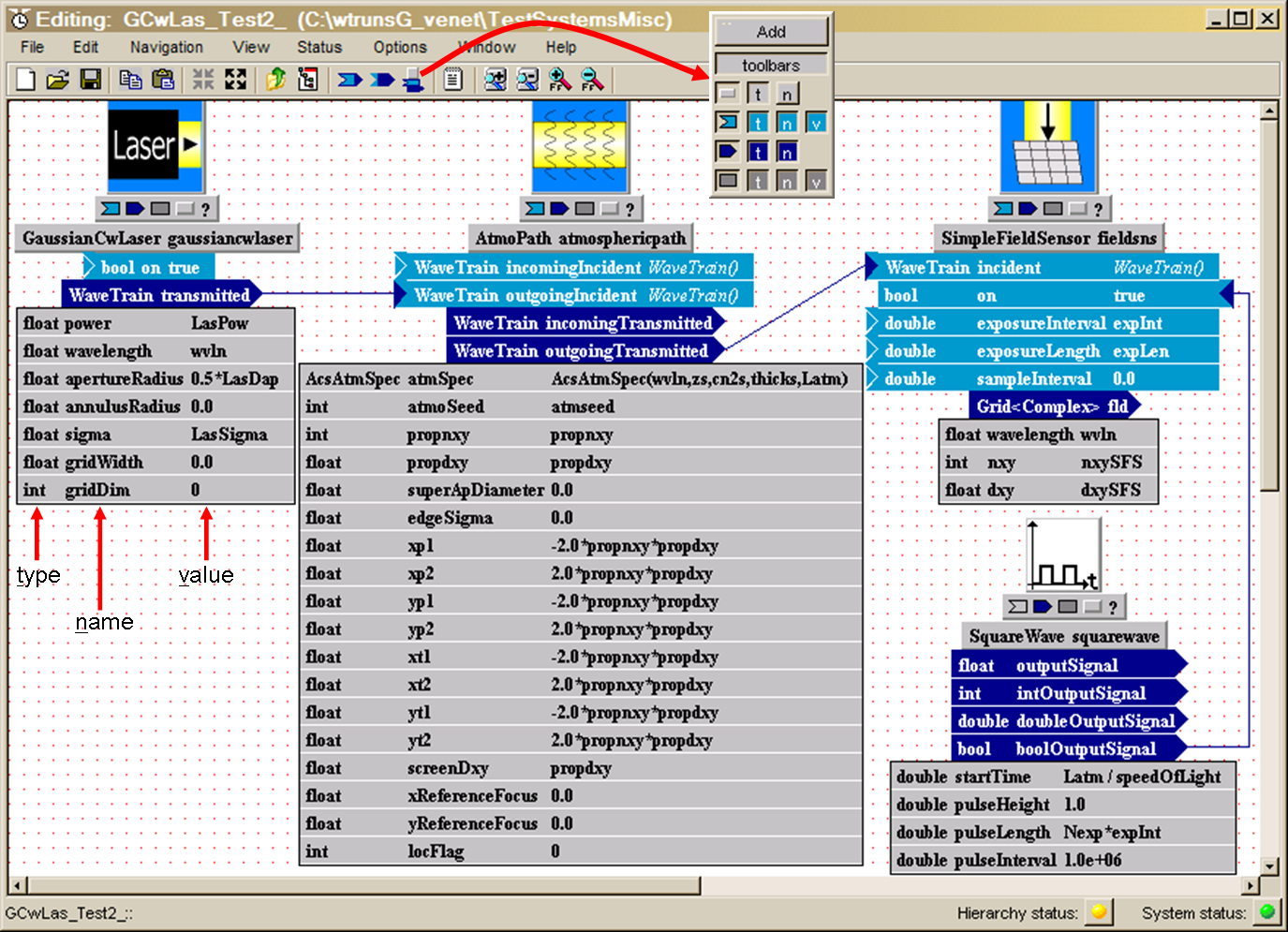
Figure: Example of data entry in the System Editor
In the System Editor blocks, the user enters data only in Value fields. To enter information, left-click in the field and type. (The following minor display deficiency may occur: prior to entering any values, it may not be obvious that a Value entry field is even present. But, left-clicking on whatever space is at the right of a line should open a little window which will then expand upon typing). The user must enter data in the parameter Value fields. The user may enter data in the input Value fields, or alternatively define inputs by connecting to the output of another subsystem. No information is entered in output lines: outputs can only be connected to inputs of other subsystems. Below we make a few further remarks on the distinctions between inputs and parameters.
In WaveTrain/tempus terminology, the entries made by the user in the Value fields are called "setting expressions". Setting expressions may consist of numerical values, user-defined variable names, or expressions. The expressions may contains a variety of algebraic operators and function names. The functions may be standard C-language math library functions, plus a variety of special WaveTrain library functions. After the user is done setting all the values, it may be more convenient for system display purposes to hide various fields and/or entire information bars, so that the display can be compacted. Hiding and unhiding information can be done one subsystem at a time, by first selecting a subsystem and then pressing the desired icon buttons; alternatively, hiding and unhiding can be done for all systems at once if no or all subsystems are selected.
The next figure shows the Run Set Editor (TRE) window for the above WaveTrain system, for a run set named "A_". This Editor also has Type, Name and Value fields, which in this case appear automatically and are labeled as such in the window itself. The Run Set Editor (TRE) window has two panels, titled "Run Variables" and "System Parameters", each of which has its own set of Type, Name and Value fields.
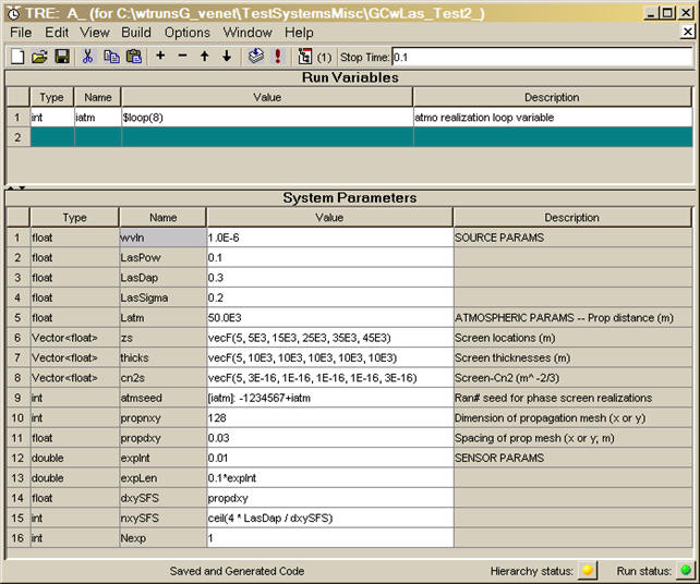
Figure: Example of data entry in the Run Set Editor (TRE)
The Type and Name columns of the System Parameter list are generated by WaveTrain, and the user must supply setting expressions for the Value fields. The Names in the System Parameter list are in one-to-one correspondence with the variables that were entered in the System Editor Value fields of the top-level WaveTrain system. For example, the name in line 1 of the System Parameters, "wvln", appears because the symbol "wvln" was entered in a Value field of the GaussianCwLaser block in the top-level system (as well as in Value fields in two other top-level blocks).
In the Run Variables panel, the user must generate the entries in all the columns. To generate any Run Variables, the user must first create an empty line by left-clicking the "+" toolbar button near the top of the Editor Window. Then, each field can be filled in. Run Variables are needed when the user wants to define loop variables, or wants to defer the numerical assignment of some of the System Parameters. It is possible to have a run set with no Run Variables at all. Deletion of Run Variables is accomplished with the "-" toolbar button, located next to the "+" button. The "" and "¯" toolbar buttons can be used to change the order of existing Run Variables (first select a line, then press the up or down button the required number of times).
Supplying entries for the Description fields in the Run Set Editor (TRE) is optional, but is very useful for purposes of future readability and documentation. To enter notes in a Description field of the Run Variables panel, simply left-click in the field and type. To enter notes in a Description field of the System Parameters panel, return to the System Editor top-level system display, select the menu option "View - Parameters", and enter the desired notes in the Description fields of that sub-window. Saving the modifications then causes the System Parameters panel in the Run Set Editor (TRE) to be updated. Note that the lines that appear in the Parameters sub-window in the System Editor (top-level system) are identical to the lines that appear in the System Parameters panel in the Run Set Editor (TRE).
Note that the Parameters sub-window in the System Editor also has "" and "¯" toolbar buttons that can be used to change the order of existing lines. There are two reasons one might want to change the order in which lines appear in the Run Variables or System Parameters panels: (1) user organizational reasons, i.e., the grouping of logically related names in whatever order makes sense to the user, (2) order requirements when values (setting expressions) are constructed in terms of other names.
"Input/parameter" distinctions
The interface of WaveTrain/tempus components consists of "inputs", "outputs" and "parameters". These are color-coded in the System Editor by the light blue, dark blue, and grey bars below the component icon picture. The "inputs" and "parameters" are both inputs in a generic sense: the distinction made in WaveTrain/tempus is that "parameters" are fixed in time, whereas "inputs" may change with time.
As far as System Editor usage is concerned, the distinction is that the user must enter a setting expression for every "parameter", but not necessarily for every "input". For "inputs", the user often has the choice of (1) entering a setting expression, or (2) defining the "input" by connecting it to an "output" of another subsystem block. Method (2) would be used if we want the "input" to vary dynamically during the execution of the simulation according to the action of the other system blocks. It is allowed to connect an "input" to another subsystem's "output" and yet to also enter a setting expression for that same "input". In that case, the setting expression is interpreted as a default value, which will be used only prior to the first instant that the other subsystem generates output. Once the other module has begun generating output, that always overrides the "input" 's setting expression.
As an example, an incident wavetrain is always a module "input", and is always defined by a connection to another subsystem (never by a setting expression). On the other hand, a tilt vector or transverse OPD array may appear as a subsystem input or parameter, depending on the component creator's ideas about how the tilt or OPD would be used in that particular module. Furthermore, even if a quantity appears as an "input" and thus allows a time-varying input to be provided, it is often perfectly logical in a particular application to define the "input" via a constant setting expression. This applies particularly to sensor exposure interval and exposure length settings, which are classed as "inputs" in WaveTrain.
In the documentation, we will try to observe the WaveTrain distinction between "inputs" and "parameters". However, for brevity we may sometimes refer to inputs in the generic sense; hopefully the meaning will be clear from the context.
Copy/Paste for text editing:
To expedite text editing in the WaveTrain Editors, copying and pasting is enabled via the mechanisms of (1) text selection with the mouse, then (2) copying and pasting using the keyboard <ctrl>-C and <ctrl>-V functions.
In order to provide the proper
setting expressions, the user must have some
awareness of the different data types used internally by WaveTrain.
WaveTrain tells the user in two places what the type assignments are:
(1) In the System Editor, the module inputs and parameters have a "type" field,
which comprises the leftmost column in the pull-down fields. (Recall that
individual columns of the input and parameter fields may be hidden or displayed
at user discretion using options on the Editor window toolbar).
(2) In the Run Set Editor (TRE), the left-most column of the System Parameters panel
automatically reports the type of those parameters that have been elevated to
the top level. In the Run Variables panel, all entries are user defined,
so here the user must enter the type as well as name and value of any desired
variables.
The principal WaveTrain data
types are
int
float
double
bool
char*
Vector<T> , where
T
= float or
complex.
Grid<T> , where
T
= float or
complex
GridGeometry
WaveTrain
Recallable<float>
DMModel&
int, float (single precision floating point), and double (double precision floating point) are the usual types of scalars encountered in programming languages. Double precision in WaveTrain is generally reserved for time variables, whereas lengths, angles, velocities, complex field and irradiance, and most other physical values are defined in single precision. The rationale for making the time variables double precision is to preserve accuracy when small time increments are added or subtracted from a relatively large running time count.
The bool (boolean) type designates a two-valued variable which can be assigned the values true or false. Variables of type bool occur in the parameter or input lists of numerous WaveTrain modules.
The char* type denotes a string variable. Note that the trailing asterisk in char* is part of the type designation. No WaveTrain modules have parameters of this type. However, WaveTrain functions that read data from external data files have string arguments that specify file names and variable names within the files. When working with these arguments, it is sometimes useful to first insert a symbolic name instead of the string that contains the actual name. This symbolic name is then of char* type, and eventually must be assigned an actual string value higher up in the hierarchy. To enter a value for a char* variable, type the string inside double quotes, as in "string".
The meaning of Vector is self-evident. Various procedures for creating and loading Vectors are described later in this chapter.
The Grid type is a special WaveTrain data construct that appears fairly frequently. Many WaveTrain modules require 2D array input data, or produce output data of that type. Examples might be an apodization map that is to be applied to an incident wave, or a sensed irradiance map. Such 2D array data in WaveTrain is organized as a special data construct called a "Grid". The Grid is another instance in which an existing mathematical term has been assigned a specialized meaning in WaveTrain. Generally in math and physics, a grid is understood to be a lattice or mesh of points on which the values of some discrete function are defined. In WaveTrain, the term Grid signifies a data structure that comprises both the coordinates of the mesh and the values of a function defined on that mesh. Procedures for creating and loading Grids are described later in this chapter.
The GridGeometry type is a special WaveTrain data construct that defines an x-y lattice of points. In many WaveTrain modules, the user specifies a lattice by simply entering scalars {dx,dy,nx,ny}, but in other cases the user is allowed more control over the registration of the lattice with respect to the x and y axes. In the latter cases, the GridGeometry data type is used. The registration of the lattice with respect to the x and y axes, and the data entry syntax for variables of type GridGeometry are described later in this chapter. Note the distinction between GridGeometry and the previously discussed type Grid: a variable of type GridGeometry defines only a lattice of points, whereas a variable of type Grid defines both a lattice and function values on the lattice.
The WaveTrain type is a special WaveTrain data construct that contains the complex values of the optical field and miscellaneous auxiliary data. The user does not need to know the properties of this structure.
The Recallable<float> type occurs in the inputs of a few WaveTrain modules. If the user supplies a setting expression to define the value of such an input, then a special function must be used in the setting expression. If the user defines the value of such an input by connecting to the output of another WaveTrain module, then that output must also be of Recallable<float> type.
The DMModel& type is a special WaveTrain data construct that appears in DeformableMirror and one or two other WaveTrain modules. Note that the trailing ampersand in the type name is part of the type designation.
---------------------
WaveTrain ver. 2007B and later:
To enable the reading of Wavetrain input data from Matlab *.mat files,
the user must explicitly tell WaveTrain the location of a particular code
library. To do this, carry out the following steps:
(a) in either the System Editor or the Run Set Editor, execute the menu sequence
"Options -- Customize TVE -- select C++ code"
(b) this causes the appearance of a code box: enter the following statement in the box.
#include "mli/mliIO.h"
(c) Press "OK" to exit the box.
If these steps are performed once, the include specification will be present in all
future
WaveTrain runsets.
This is the only user-added include statement that is necessary as of v2007B.
---------------------
---------------------
WaveTrain versions 2007A or older:
To enable the execution of many of the data-entry procedures described in the present chapter, the user must explicitly ensure that WaveTrain has access to several code libraries that are provided in the WaveTrain/tempus suite. This requires the entry of some information in the "C++ code box" in the Run Set Editor (TRE). (In future versions of WaveTrain, this will be done by default, but at present the user must enter these directives manually). The following instructions assume that the user has created a Run Set for a WaveTrain system.
If the user has an older version of the WaveTrain GUI, the "C++ code box" should be immediately visible at the upper right of the Run Set Editor (TRE) main screen. Most users will have a newer version of the GUI, in which the C++ code box is opened by pulling down the "Edit" menu, then selecting "Edit C++ Code". Now the user should type the following lines in the C++ code box, using exactly the syntax shown:
#include
"TempusInitializers.h"
#include "mliIO.h"
#include "math.h"
#include "MathematicalConstants.h"
#include "PhysicalConstants.h"
 The
appearance of the C++ code box in the newer GUI versions is as shown at right.
After entering these commands, the code box can be closed (in the newer GUI) and
the Run Set saved. When the Run Set is compiled, these directives will
enable the compiler to find various functions and constants that are discussed
below. Even if the user's run set and system make no immediate use of
these libraries, we recommend that the user always enter these include
directives as a standard part of any run set construction. That way, any
potentially needed function or constant will be available for future use,
without further ado.
The
appearance of the C++ code box in the newer GUI versions is as shown at right.
After entering these commands, the code box can be closed (in the newer GUI) and
the Run Set saved. When the Run Set is compiled, these directives will
enable the compiler to find various functions and constants that are discussed
below. Even if the user's run set and system make no immediate use of
these libraries, we recommend that the user always enter these include
directives as a standard part of any run set construction. That way, any
potentially needed function or constant will be available for future use,
without further ado.
---------------------
(REMINDER: To ensure the availability of all the constants discussed in this subsection, the reader should review the earlier section regarding include setup.)
WaveTrain has built-in names for a few special constants that are frequently needed in setting expressions:
speedOfLight: The speed of light is frequently needed to define time delays in sensor triggering. The value supplied by this WaveTrain symbol is the speed in vacuum. This is sufficient for WaveTrain purposes, since continuous media are represented by the split step method of vacuum propagation between phase screens. In this propagation model, the actual speed of light in a medium is never used.
PI: the number p.
TNANQ: the special numerical value NotANumber. This symbol is required in a few WaveTrain systems to force unconnected inputs to be ignored. The more usual notation of plain "NaN" will not work. (It is possible that users may encounter "NaN" as a default setting expression in some older modules; if so, this is a residual code bug, and the user should change the value to "TNANQ".)
C-language syntax for expressions and basic math functions
(REMINDER: To ensure the availability of all the functions discussed in this subsection, the reader should review the earlier section regarding include setup.)
When the user completes assembly of a WaveTrain run set, and then presses the "Compile and Link" button on the editor toolbar, the initial (behind-the-scenes) result is the generation of a C++ source-code file. Since C++ is the underlying language of the WaveTrain code suite, much of the syntax used in setting expressions follows C rules.
Variable names, numbers, scalar operators and expressions:
Variable names used in setting expressions may contain any letter (upper or lower case), the numerals 0-9, and the underscore. The first character of a name should be a letter. Names are case sensitive.
Numbers of type float or double may be entered in purely decimal form or in the exponential format, sx.xEsn, where s is an optional sign. The E symbol can be entered in lower case, if desired. Numbers of type int are 32-bit signed integers, meaning that the allowed values range from -231 to 231-1.
The usual scalar operators {+, - , *, /} are supported. When a setting expression contains algebraic formulas, the user should be aware that C type conversion rules will be followed when the expression is evaluated. The main caution to be observed in this regard is illustrated by a setting expression such as (1/n)*f. If n is of type int, then evaluation of (1/n) will cause an undesired result if the user actually meant for (1/n) to be evaluated using floating-point rather than integer arithmetic. To avoid this kind of error, we recommend that users always enter the literal constants as 1.0, etc., in algebraic expressions. Integer truncation or round-up, if desired, can be achieved using functions from the standard C math library.
A setting expression may refer to an element of a previously defined vector using the bracket notation that is used in C syntax. For example, the setting expression v[4] signifies the 5th element of a vector v that was defined in a previous line of the Run Set: note that the example refers to the 5th element because C indexing is 0-based.
Standard C math library functions:
The following standard C library functions may be used when entering setting expressions in the Run Set Editor (TRE) or System Editor windows. Note that only scalar arguments are allowed:
sin(x), cos(x), tan(x)
asin(x), acos(x)
atan(x): range [-p/2,
p/2]
atan2(y,x):
range [-p,
p]
sinh(x), cosh(x), tanh(x)
exp(x), log(x), log10(x)
pow(x,y): the power function xy
(the caret notation x^y is NOT allowed)
sqrt(x)
ceil(x), floor(x): the smallest- and
greatest-integer functions, respectively
fabs(x): the
absolute value |x|
fmod(x,y):
floating-point remainder of x/y, with same sign as x.
The Run Set Editor (TRE) allows the definition of loop indices. A loop index may be defined in the Run Variables panel of the editor; then, an existing variable that controls a system parameter is defined in terms of the loop index. A loop index will cause WaveTrain to execute the simulation once for each value of the loop index, and will store all recorded results in the same .trf file. If more than one loop index is defined, a set of nested loops will be executed, with the nesting order being the order in which the loop indices are defined in the Run Variables panel. The uppermost loop index in the panel's list of variables is the outermost loop index. Loop indices may appear anywhere in the Run Variables panel, interspersed with non-loop variables. It is perfectly acceptable for a run set to have no loop indices. Note that the user does not supply a loop index corresponding to the time steps of the simulation: the time steps are all defined by sensor triggering and timing specifications together with the StopTime.
WaveTrain uses the following terminology: the aggregate of simulation executions over all loop variables is called a run set, whereas the execution for one realization of the loop variables is called one run. Each run contains the number of time steps determined by sensor timing specifications and the simulation StopTIme. The output data for the entire run set is stored in one trf file. Before defining too many loop variables, the user should remember that even a single run can generate very large amounts of data, particularly if the simulation has many time steps with recording of 2-D data at each time step.
An example of loop index usage is given in the previous
illustration of a run set. The
usage comprises two steps, each requiring a special syntax:
(1) We have created a Run Variable of type
int, named
iatm. Then we entered
the setting expression
$loop(N), where
N is 8 in the illustration, to define the number of
times that the loop should be executed. This action defines a loop index
variable iatm
that will cycle through the values 0,1,...,N-1.
(2) After defining the loop variable, we can use it in another setting
expression that defines the value of a System Parameter (or possibly another Run
Variable) in terms of the loop index variable. In the illustration, line 9
of the System Parameters assigns the value of
atmseed in terms of an algebraic expression that
involves the loop index iatm.
NOTE the special prefix [iatm]:
required in the setting expression when the loop index is used.
The argument of a $loop(N) expression may be a constant or a previously-defined run variable.
As mentioned above, each value of the loop index results in one "run" over the number of time steps that have been defined, and the recorded outputs from all runs are stored in a single .trf file. If there are two loop variables, there will be one run for each ordered pair of loop indices, etc. Details on reading the .trf data are given in another section of this User Guide.
To specify what simulation outputs will be recorded in the .trf file, the user must open the Output Recording menu and check the boxes associated with the desired variables. The following picture illustrates the procedure:
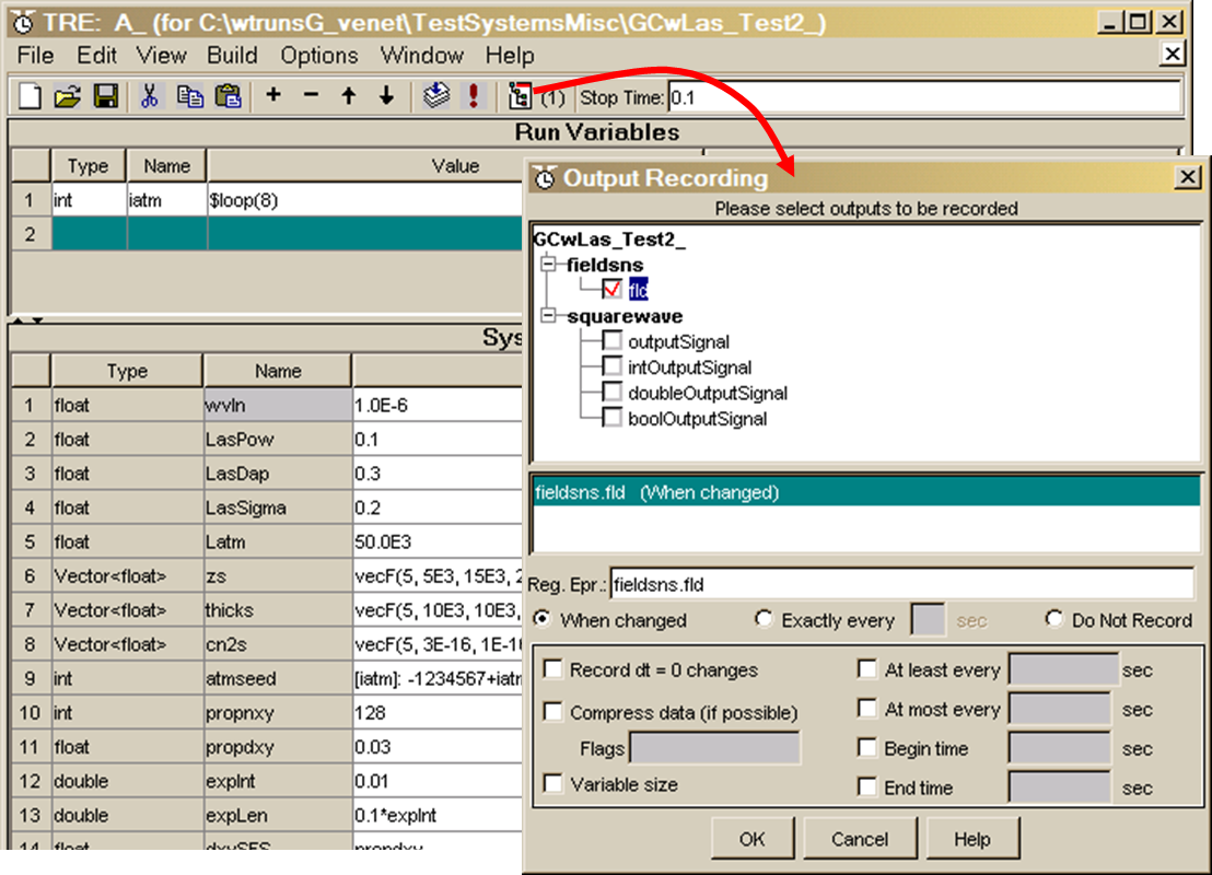
The Output Recording menu is opened by left-clicking a toolbar button in the RunSet Editor, as indicated by the curved red arrow in the picture. This causes the Output Recording menu to appear; the menu illustrated here is the one associated with our previous example system and run set. In the top panel of the menu we see a tree-format list, organized by subsystems, showing all the Outputs of the WaveTrain subsystems that comprise our system. "Output" here is used in the technical WaveTrain sense, signifying those quantities that appear in the dark blue bars attached to all the subsystem icons. (We said that "all Outputs" are listed, but comparison of the Recording menu and the System Editor shows that "all" actually means all except the Outputs of data type WaveTrain. Outputs of that data type cannot be recorded directly.) The items in the Output Recording list are the only computed quantities that can be recorded during a simulation run. The illustrated list is quite short because our example system is simple. In the illustration, we have checked only one Output for recording, namely the complex field (fld) measured by the SimpleFieldSensor subsystem. The selected items are indicated by the red check marks. Note that a simulation will not run unless at least one Output is checked for recording.
The middle panel of the Output Recording menu simply shows a sequential list of all the selected variables.
The bottom panel in the menu shows various timing options. These options work together with the sensor subsystem timing parameters and the SquareWave triggering mechanism explained in another Guide section. Unless some unusual need arises, we recommend for simplicity that users always choose to record "When changed": in conjunction with the sensor timing and triggering, this is sufficient for essentially any situation.
Procedures for entering vectors, arrays and "Grids"
(REMINDER: To ensure the availability of all the functions discussed in this subsection, the reader should review the earlier section regarding include setup.)
There are two general methods
available for entering vector, array and Grid data:
(1) Use WaveTrain library functions to create certain simple data (a
vector of all ones or zeros, or a Grid of ones, for example).
(2) Use WaveTrain library functions to read arbitrary data from
Matlab-generated *.mat data files.
These two methods are available when entering
setting expressions in the Run Set Editor (TRE), or in the System Editor (i.e., in
the pull-down value fields of WaveTrain library modules).
Two companion documents list all the relevant library functions, and fully define the calling syntax. These two "documents" are actually source code header files, but the files consist mostly of readable documentation: the files are TempusInitializers.h and mliIO.h. The principal options are explained in the examples below: if different options are desired, users should scan the two *.h files for the availability of options not documented below.
The library functions calls documented in the present subsection may be entered as setting expressions in the Value fields of the Run Set Editor (TRE), or in the Value fields of subsystem modules in the System Editor. The illustrations in the present subsection happen to all show entries in subsystem modules, but the syntax is identical when entering the function calls in the Run Set Editor (TRE).
Using library functions to create vectors, arrays and Grids
Example 1 (vectors):
Consider the module
BeamSteeringMirror, which will be a key component in most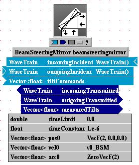 tilt-tracking systems. As we see in the figure
at right, the last three parameters, named pos0,
vel0, and acc0 are of type
Vector<float>. Together, these constant vectors specify the initial
state of the mirror. To assign values to these
quantities, we must enter a two-vector specifying the
x and y components in each value field. A relevant function from the
TempusInitializers.h
set is
tilt-tracking systems. As we see in the figure
at right, the last three parameters, named pos0,
vel0, and acc0 are of type
Vector<float>. Together, these constant vectors specify the initial
state of the mirror. To assign values to these
quantities, we must enter a two-vector specifying the
x and y components in each value field. A relevant function from the
TempusInitializers.h
set is
VecF(2,x,y)
,
where 2 specifies the length of the vector, and x and y are the desired
component values. This is shown entered into the value field of pos0
in the figure as
VecF(2,0.0,0.0). Note that
the general function form
VecF(n,v1,v2,...)
is limited to n<=10. Since in this case we
wanted to specify a zero vector, an alternate procedure would have been to enter
the function
ZeroVecF(2).
This is illustrated in the figure as the value assignment for acc0.
Finally, in the case of vel0, we assigned a value by entering the
symbolic name v0_BSM, with the understanding that this symbol is
"elevated" as a parameter name of the next higher block diagram level. At
some level up the chain, the name must be assigned a value, using the same
procedure that we illustrated for pos0 and acc0.
Reading through TempusInitializers.h, the user can see that different functions exist for creating vectors of integer, float, double, and complex type. The function type must be matched to the type of the variable as it appears in the type field of the module in question. Also, there are specific functions for creating constant vectors and several other special formats.
Summary list of vector creation functions: The following is a complete list of the available vector creation functions. The general usage principles are always identical to the examples given above. Frequently, for a given "F" function that creates a float type, there are parallel "I", "D", and "C" functions that create, respectively, an integer type, a double type, and a complex type. For definitions and argument syntax of each function not explained above, consult the file TempusInitializers.h:
VecF
(or I); CAUTION: VecF and VecI are limited to lengths
≤ 10.
ZeroVecF (or I, or D, or C)
OnesVecF (or I, or D, or C)
ConsVecF (or I, or D, or C
IndexVecF (or I, or D)
PokeVecF (or I, or D)
TwoVecF ( or D)
NanVec
MeshXVecF, MeshYVecF
Example 2 (Grids):
Consider the module FixedOpdMap,
which is used to apply a static 2D phase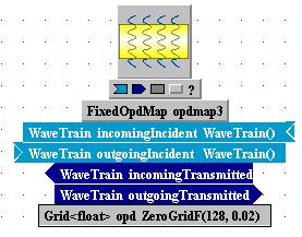 retardation to an incident wavetrain. As shown in the figure at right, the
parameter opd is of type Grid<float>. This signifies the
special WaveTrain Grid construct that was
defined above. Again referring to
TempusInitializers.h,
we see that functions exist for the creation of uniform Grids of ones or zeros,
of type float or complex. For example, assigning the value
retardation to an incident wavetrain. As shown in the figure at right, the
parameter opd is of type Grid<float>. This signifies the
special WaveTrain Grid construct that was
defined above. Again referring to
TempusInitializers.h,
we see that functions exist for the creation of uniform Grids of ones or zeros,
of type float or complex. For example, assigning the value
ZeroGridF(128, 0.02)
creates a grid of (nx=128)x(ny=128) zeros, with a grid spacing dx=dy=0.02 m in
each dimension, and with the (nx/2,ny/2) point at (x,y)=(0,0). At this
level, we are dealing with C-language code, so index n/2 is to be interpreted as
0-based.
Alternate syntax:
the grid creation functions such as ZeroGridF
and OnesGridF have an
alternate syntax that uses the special WaveTrain
data type GridGeometry. This alternate syntax allows more freedom in
specifying the offset of the mesh points with respect (x,y)=(0,0), which is
sometimes necessary. Recall that in the above example we stated that the
(nx/2,ny/2) point necessarily lay at (x,y)=(0,0). By expressing the
argument syntax as, for example,
OnesGridF(gwoom(nx,ny,dx,dy))
or
OnesGridF(GridGeometry(nx,ny,dx,dy)),
we can define the position of the mesh points on which the grid is defined more
generally. This syntax uses yet more special WaveTrain functions, namely
gwoom(...) and GridGeometry(...), which are
explained in the linked section.
The library functions available for Grid creation are limited to the creation of spatially uniform Grids of ones or zeros. The section on modifying vectors and Grids shows how to extend this to uniform grids of any constant value. In order to input a more general spatially-varying Grid, we must use a library function that can read a Grid from a *.mat file. This procedure is explained in the section immediately following.
Note on interpolation: When inputting Grids, either by the function method or by the reading-from-file method, it is important to understand that WaveTrain will automatically interpolate the data Grid onto the propagation mesh or onto whatever computational mesh is relevant to the module that uses the Grid. In the case of FixedOpdMap, for example, the module's math operation is to multiply the incident wavetrain by a unit-magnitude phasor constructed from the input opd. Since the incident wavetrain values are specified on the propagation mesh, WaveTrain interpolates the opd Grid onto that propagation mesh in order to do the phasor multiplication. The interpolation capability is an important convenience for the user: without this feature, the user would constantly need to recreate possibly complicated input maps every time the propagation geometry changed.
Using library functions to read scalars, vectors, arrays and Grids from *.mat files
Example 1 (vectors): Consider the module Tilt, which adds a specified tilt to an incident wavetrain. As illustrated in the figure below, the module has an input called tilt, which is a two-vector of float type.
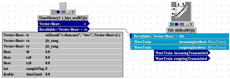
The tilt type field also
indicates the property "Recallable": we'll return briefly to that
complication at the end of the example. While a static tilt
two-vector could be input in the value field of the Tilt module, that is a
trivial example. A more practical problem would be to input a user-defined
sequence of tilts that represents, for example, one temporal realization of a
correlated random mount jitter. To achieve this end, the figure shows
Tilt preceded by a TimeHistory2
module. TimeHistory2 outputs at any instant a Recallable vector of length
two, which is connected to the tilt input of the Tilt module. The
key point for our example is that TimeHistory2 has three input parameters that
specify the temporal evolution of the output two-vector that becomes the
instantaneous tilt
increment: the three relevant parameters are tv, vx, and
vy. Each of these three are themselves n-vectors that together specify
the desired time sequence: that is, [vx(i), vy(i)] will define the desired
tilt at simulation time t(i). The procedure for creating and importing the
tv, vx, and vy vectors is:
(1) Using Matlab, create the sequence of vectors satisfying the desired
physical criteria.
(2) Save the vectors in a *.mat file.
(3) Read the vectors into WaveTrain using the function
mliLoad(...). The
function syntax is fully defined in
mliIO.h, and the specialization
to the present example is as follows. Suppose that: (a) the name of
the *.mat file is c:/data.mat, and (b)
tvec is the name of the vector variable in the data file that we want to
associate with tv. Then we could enter the following syntax into
tv's value field, as illustrated in the figure:
mliLoad("c:/data.mat", "tvec",
Vector<float>())
The usual "./" and "../" directory abbreviations may be used in specifying the
file path.
Unless otherwise specified, the vector variables in the *.mat file may be
row or column vectors.
Analogous
mliLoad commands could be
entered in the value fields of the vectors vx
and vy. Alternatively, we could enter symbolic names in the value
fields, as the above example illustrates for the case of vx
and vy.
These symbols are "elevated" as parameter name of the next higher block diagram
level. At some level up the chain, the names must be assigned actual
values, either by using the
mliLoad command or one of the
creation functions discussed previously.
Note that the mliLoad operation extracts specified variables from the external data file by name (tvec in our example). Therefore, the external *.mat file may contain any other data in addition to the data required for any particular mliLoad operation. This allows the user to group data in various ways convenient to the overall problem.
The "Recallable" property: The present example involves a variable which has the special designation "Recallable". Recallable variables, and some special usage rules required for such variables, are discussed more fully in another section. In the present example, all Recallable issues are handled automatically, and the user need not be concerned with any special usages. TimeHistory2 uses its input data to create a Recallable vector, and passes that to Tilt, which requires a Recallable input tilt, so all the types match without further ado.
(Side note: The module TimeHistory2 has an important interpolation feature. It would be quite inconvenient if the time sequence tv needed to match exactly the discrete time instants of the simulation run. Therefore, WaveTrain automatically interpolates tv, vx, and vy as needed for whatever the time instants of the simulation are. The user should not, however, attempt to make WaveTrain extrapolate. This is analogous to WaveTrain's automatic spatial interpolation that we discussed in the preceding example of inputting a Grid.)
Scalars: Although less necessary than reading vectors and Grids, it may also be convenient to read certain scalar values from *.mat files. To do so, the mliLoad format is simply mliLoad("c:/data.mat", "varname", float()).
Example 2 (Grids):
Consider once again the module
FixedOpdMap, which is used to apply a static 2D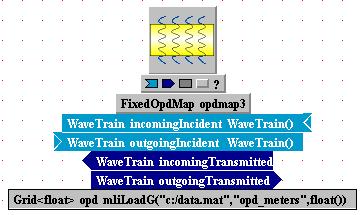 phase retardation to an incident wavetrain. As discussed in the previous
example related to Grids, the parameter opd is of type Grid<float>.
In the previous example, we saw how a library function could be used to quickly
create and set values of simple uniform Grids. This is useful, but of
course very limited. To work with Grids whose function values have an
arbitrary spatial dependence, the procedure is:
phase retardation to an incident wavetrain. As discussed in the previous
example related to Grids, the parameter opd is of type Grid<float>.
In the previous example, we saw how a library function could be used to quickly
create and set values of simple uniform Grids. This is useful, but of
course very limited. To work with Grids whose function values have an
arbitrary spatial dependence, the procedure is:
(1) Using Matlab, create a structure variable with three fields, s.x,
s.y, s.g, that has the physical parameters of the desired Grid:
s.x = row vector(1:nx), values of the
x-coordinates of a rectangular lattice of points
s.y = row vector(1:ny), values of the
y-coordinates of a rectangular lattice of points
s.g = array(1:nx, 1:ny), values of a
function on the nx
´
ny lattice.
The name s can be arbitrarily chosen, but the fields must be named .x,
.y and .g.
(2) Save the structure variable in a *.mat file.
(3) Read the structure variable into WaveTrain as a Grid using the
mliLoadG(...) function.
Suppose that: (a) the name
of the *.mat file is c:/data.mat, and (b) opd_meters
is the name of the structure variable in the data file. Then we could
enter the following syntax into FixedOpdMap's opd value field, as
illustrated above:
mliLoadG("c:/data.mat","opd_meters",float())
The usual "./" and "../" directory
abbreviations may be used in specifying the file path.
There is an analogous syntax for loading a
complex-value Grid, if a WaveTrain component requires that:
mliLoadG("matFilePath","matStrucName",Complex()) .
In this case, the array s.g must contain (nx)*(ny) complex values
as generated in Matlab.
Variations on the above procedure are also available, and are detailed in the companion documentation mliIO.h.
To conclude this example, we remind the reader of the important spatial interpolation feature that is applied to data Grids: this was discussed in more detail in the previous examples. Grid input procedures are quite important, since there are many examples of modules other than FixedOpdMap that require loading of a Grid. A few important examples are the Apodizer module, the rough reflector modules (e.g., CoherentTarget), and the SensorNoise module.
Using library functions to read a complex Grid from a text file
The available library functions for inputting data from files are mostly dedicated to reading from *.mat files. However, there is at least one library function available for loading data from plain text (ASCII) files.
The available function can be used to input a
Grid<Complex> by reading the real and imaginary array parts from two separate
plain-text files. The setting expression syntax is:
where
reFile (imFile) should contain a tab-delimited array of numbers corresponding to the real (imaginary) part of the Grid values, and where nx,ny,dx,dy specify the mesh dimensions and physical spacing (MKS units). x should correspond to the first dimension (i.e., down-column). The FileGridC function would be used in the same context where the function mliLoadG("matFilePath", "matStrucName", Complex()) could be used (as illustrated in the section dedicated to reading from *.mat files).
From time to time, further functions for loading data from text files may be added to the WaveTrain capabilities. Users can check the file TempusInitializers.h in their WaveTrain installation to see if any new read syntaxes have been added since the User Guide was updated.
Procedures for modifying vectors, arrays and "Grids"
When constructing setting expressions, it is sometimes desirable or convenient to construct linear combinations of vectors or of Grids. This requires some caution in the WaveTrain GUI, because the ordinary arithmetic operation symbols { +, -, *, / } are defined for certain combinations of mixed scalar, vector and Grid arguments but not others.
We emphasize that the procedures discussed in the present subsection are only relevant to the construction of setting expressions. By way of contrast, there is also a different context in which various linear combinations of vectors are supported: there exist WaveTrain library modules that can, for example, add vectors (SumVFD), or multiply a vector by a scalar (Gain). Although these systems could be inserted into a WaveTrain system to accomplish at least some of the actions illustrated below, that would be a tedious and unnatural alternative. Those library modules are principally meant to handle operations when the vectors of interest are changing with time, rather than just being static input parameters. (The referenced library modules, and other of a similar nature, can be found in the ControlsLib subset of wtLib. Also, ProcessingLib may contain a few additional modules of this type, although mainly ProcessingLib components comprise more complex operations.)
CAUTION: The modification procedures documented in the present subsection may be used only in the Value fields of the Run Set Editor (TRE), but not in the Value fields of subsystem modules in the System Editor.
General linear combination of vectors
The ordinary arithmetic operation symbols { +, -, *, / } support the formation of linear combinations of vectors. That is, the syntax s1*v1+s2*v2 is supported, where {s1,s2} are scalars and {v1,v2} are vectors. (The operators {- , /} may be used in the analogous way.) The following excerpt from a WaveTrain run set illustrates:
The final line of the excerpt defines a variable called vys_, of type Vector<float>. This variable is defined in the Value field as a linear combination v1+s2*v2, where the vector v1 = vys_wind and the vector v2 = hscreens were defined in previous lines (12 and 5, respectively) of the excerpt. The scalar s2 is itself a composite of several previously-defined scalars in this example.
CAUTION: linear combinations formed directly with vector-creating library functions are not allowed. For example, consider run variable 5, where vector hscreens is defined in terms of the data-loading function mliLoad(...). Although in an operational sense the mliLoad call does return a vector, it is not allowed to directly form, e.g., the setting expression 3.0 * mliLoad(...). In order to form linear combinations with the vector defined by the mliLoad(...) call, it is necessary to define a succession of run variables, as illustrated in the above excerpt.
Multiplying or dividing a Grid by a scalar
In the case of a Grid, multiplication or division by a scalar means that the Grid's *.g field is to be scaled by the constant, but the *.x and *.y coordinate vectors are to be left unchanged. For a Grid operand, use of the ordinary arithmetic operation symbols { +, -, *, / } is not supported. The following excerpt from a run set illustrates a special syntax that must used to accomplish the scaling:
In this example, we
have a system parameter named respWfs, of type Grid<float>. In the
Value entry field, we have entered a compound setting expression that consists
of two successive expressions separated by a semicolon:
First expression: We begin by using the WaveTrain
library function OnesGridF(...) to
set respWfs equal to a Grid whose *.g
values are 1.0 at every mesh point. The Grid has (x,y) dimensions 64x64,
and the mesh spacing is 0.01m. In general, this first statement in the
setting expression can follow any of the patterns previously allowed for Grid
definition.
Second expression: After the semicolon, we can add a second
statement that modifies the initial definition of respWfs. In this
case we want to multiply the Grid by the number 11.0, but the ordinary
arithmetic operator " * " is not supported for a Grid operand. Instead,
the desired multiplication is achieved by using the " *= " syntax shown in the
example. This syntax may be familiar to C/C++ users. Instead of
entering a literal constant like 11.0, we could have entered a previously
defined variable name. Notice how the type of the scalar factor ("float",
in this case) should also be declared.
The { *=, /=, ...} operations illustrated above for modifying a Grid can also be applied to vectors. However, since the more natural use of the usual operators { +, -, *, / } is supported for vectors, as illustrated previously, there is generally no need to resort to the " *= " type of syntax when forming linear combinations of vectors.
The functions "gwoom" and "GridGeometry"
(REMINDER: To ensure the availability of all the functions discussed in this subsection, the reader should review the earlier section regarding include setup.)
In the summary section on data types, we introduced the data type called GridGeometry. The central idea was that a variable of data type GridGeometry defines the coordinates of a rectangular lattice or mesh of points. In various WaveTrain library systems, it is necessary to specify setting expressions that define a lattice of points. Frequently this can be done by simply entering scalars (nx,ny,dx,dy) or (nxy,dxy), but in other cases the user is allowed more control over the registration of the lattice with respect to the x and y axes. In the latter cases, the GridGeometry data type is used, in conjunction with the functions gwoom(...) and GridGeometry(...). As explained in an earlier section that introduced discrete mesh specifications, the main feature that distinguishes the two mesh-definition functions is the grid offset. The user may wish to review that referenced section at this time. The remainder of the present section gives illustrations of the syntax to be used when meshes are specified using the gwoom(...) and GridGeometry(...) functions.
gwoom syntax
There are two argument options: the first allows specification of an asymmetric mesh, and the second allows only a square mesh:
(1)
gwoom(nx,ny,dx,dy): the
integers nx,ny are the mesh dimensions, and the floating-point constants dx,dy
are the mesh spacings, in meters.
(2) gwoom(nxy,dxy):
integer nxy is the mesh dimension, in either x or y, and dxy is the mesh spacing
in meters.
The alternate function name grid_with_origin_on_mesh(...) may be used instead of gwoom(...); the first letters of the expanded name also explain the source of the "gwoom" name.
GridGeometry syntax
There are several argument options. The first two are identical to the gwoom options:
(1)
GridGeometry(nx,ny,dx,dy):
the integers nx,ny are the mesh dimensions, and the floating-point constants
dx,dy are the mesh spacings, in meters.
(2) GridGeometry(nxy,dxy):
integer nxy is the mesh dimension, in either x or y, and dxy is the mesh spacing
in meters.
The above two function argument options are the only ones needed to produce grid offsets of the type described in the introductory section on discrete mesh specifications. These options suffice for almost all cases. However, occasionally a completely general offset is desired, and this can be achieved with the following function argument option:
(3) GridGeometry(RectangularRegion(xmin,xmax,ymin,ymax),dx,dy): in this option, the user specifies the physical coordinates of the mesh corner points, and the dx,dy spacings. RectangularRegion is itself another WaveTrain library function; the corner coordinate and spacing arguments can be replaced by literal constants or symbols that can be elevated (promoted) up the hierarchy as usual.
Subsystem usage examples
Consider the library system SensorNoise. An important function of this system, entirely separate from generating noise, is to carry out spatial integration of an input (usually irradiance) map. In SensorNoise, the new mesh defines the centers of the physical pixels over which the input is spatially integrated. In modeling applications like wavefront sensors, it may be critical to precisely define the registration of a physical-pixel mesh with respect to the input data mesh. In such cases, one needs to carefully apply the gwoom or GridGeometry functions to obtain the desired result. Another section of the User Guide is devoted more to the physical issues handled by SensorNoise; in the present section, we simply use the SensorNoise block to provide examples of how and where to apply the gwoom and GridGeometry function syntax.
Consider the left panel in the following picture, which shows an isolated SensorNoise block. We are interested in the two parameters marked by the red arrows. The first parameter, named detectorGrid, is designated in column1 as being of type GridGeometry. Therefore, we must supply a setting expression in column3 that has the matching type, and we have done so by using the GridGeometry function, with the syntax "GridGeometry(nxy,dxy)". The nxy and dxy are parameters that must be elevated up the hierarchy and assigned numerical values at some level. In this manner, we have specified the mesh coordinates designated as detectorGrid: these points are the centers of the physical pixels discussed in the preceding paragraph.
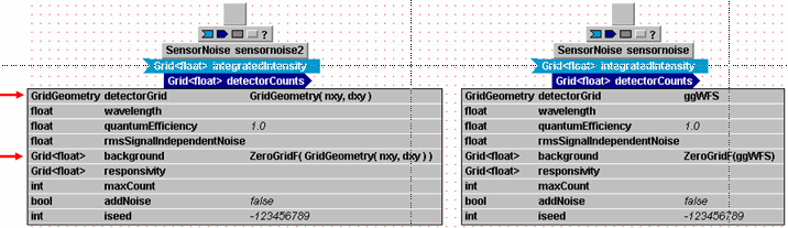
Now consider the second parameter marked with a red arrow. This is designated in column1 as being of type Grid<float>. Recall that a WaveTrain Grid is a quantity that comprises both a mesh and a set of function values on that mesh. We must supply a setting expression in column3 that has the matching type, and we have done so by using the ZeroGrid function, with a single argument that consists of a call to the GridGeometry function. Evidently, we have defined the meshes of detectorGrid and background to be identical; but remember that background comprises a set of function values (zeros in this case) in addition to the mesh. Recall also that there exist other useful syntaxes for assigning values to a Grid data type: the general introduction to specifying Grids was given in an earlier section.
The right panel of the figure is a variation that shows how we might proceed if we wanted to elevate the definition of the mesh to a higher level in the system hierarchy, or to the run set. In the case of the "detectorGrid" variable, we have simply assigned a symbolic name, ggWFS, which must be elevated (promoted) to the next higher hierarchy level. For the variable background, we assumed that we still want zero values assigned, so we kept the ZeroGridF function, but used ggWFS as the argument to specify the mesh on which the zeros exist. If we wanted to defer the assignment of the grid values as well as the mesh type, we could have simply assigned another symbol, say bgdWFS, as the background value.
Miscellaneous special functions and operators
Some WaveTrain library modules
have scalar inputs whose
type is designated as Recallable<float>.
The
Focus module shown at right
is an example. For generality, the scalar in question (the
focusDistance, in this case)
has been designated an "input" so that it can change with time. In many,
if not most, systems the user will simply want to define the scalar as constant
during the simulation run (rather than connecting some other system's output to
the
focusDistance input).
However, because of type-matching requirements, the
setting expression entered in the value field cannot be of
float
type, but rather must be explicitly defined as a
Recallable<float> type.
The picture at right shows one way of doing this, using the WaveTrain library
function recallableFloat(...).
Alternatives are to enter:
(1) recallableFloat(EFL),
as shown in the picture: this defines a variable
EFL that will be elevated as a
float type, and must then be
assigned a numerical value at a higher system level.
(2) recallableFloat(10.0):
the literal constant 10.0 is converted to recallable type.
(3) EFL:
this defines a variable
EFL that will be elevated as
a Recallable<float>
type, and must then be assigned a value at a higher system level. The
required use of the
recallableFloat(...)
function is simply deferred to the higher system level, and there is usually no
good reason for doing this.
WaveTrain components for data-type conversion
The above example, involving the function "recallableFloat",
illustrated a situation where data-type conversion is required in
setting expressions. There are analogous situations where it is
physically logical to connect a component's output to another component's input,
but the data types of the output and input
have unfortunately been defined differently. This could be as simple,
e.g., as the output being single precision (type "float"),
and the input being double precision ("double").
Another example that may crop up is integer ("int")
versus boolean ("bool").
Conversions such as these must be done using components from WaveTrain's
ConvertLib library, inserted
into the WaveTrain system in the System Editor. This procedure differs
from the previous
recallableFloat
example, where a conversion function was inserted in a setting
expression; however, the concept is similar insofar as both procedures
satisfy the need to occasionally mate different data types in the System Editor.
There are several situations in which the System Editor or Run Set Editor issue "obsolete" warnings.
(1) Obsolete components
When an existing system is opened
in the System Editor, it may happen that one or more components appear with the notation "obsolete" above the component icon.
The figure at right shows an example. This typically indicates that the
component in the user's Wavetrain installation has been updated in some way with
respect to the component in the opened system. In the vast majority of
cases, there is no real conflict implied by this: the user should simply
execute the System Editor menu sequence Edit -- Update Obsolete Subsystems,
selecting all the subsystems to be updated in the list that is presented.
components appear with the notation "obsolete" above the component icon.
The figure at right shows an example. This typically indicates that the
component in the user's Wavetrain installation has been updated in some way with
respect to the component in the opened system. In the vast majority of
cases, there is no real conflict implied by this: the user should simply
execute the System Editor menu sequence Edit -- Update Obsolete Subsystems,
selecting all the subsystems to be updated in the list that is presented.
Potentially, if a major change was made to the component interface (inputs, outputs or parameters were changed, added or removed), then the containing WaveTrain system might no longer work after updating. However, this is very unlikely: if a WaveTrain component were changed that significantly, it would be much more likely that a modified component would be added to the Wavetrain libraries (unless perhaps the old component had been discovered to produce out-and-out wrong results). By far the most likely scenario is that the change is insignificant to the user. At present, there is no simple way for the user to discover exactly what the change is that triggered the "obsolete" warning. As noted above, the default recommendation is to update.
(2) Obsolete runsets
A completely different "obsolete" situation occurs when the user makes changes in a system that affect the runset. This will occur relatively frequently in normal WaveTrain practice. This was discussed in several spots in the introductory tutorial. for completeness, we repeat the principal paragraph below.
Suppose that you have already created a run set for a WaveTrain system, and then you subsequently edit the system in the System Editor. Many such changes will temporarily render the run set invalid, and you must execute Edit - Update in the Run Set Editor window to continue working there. There should be no confusion as to whether you need to do this: the condition is signalled by the message "Obsolete" in the status bar at the bottom of the Run Set Editor, and by the inability to access various grayed-out menu options.
If a run set is not open when you edit its system, then the "Obsolete" message will appear when you next open the run set. There is no possibility of incorrectly executing the simulation run due to forgotting to perform this synchronization step.
Status bulbs and status checking
At the bottom right of the System Editor window, there are two status indicators:
![]() and
and
![]() .
.
The two colored bulbs can be either red, yellow or green, indicating various levels of missing or inconsistent information in the parameter and input setting expressions.
The "System status" bulb refers to the system level currently displayed in the Editor window. The "Hierarchy status" bulb refers to the complete level structure of the Wavetrain system. For example, it is possible that: (i) a component in the current window is a composite system that itself contains other library components, or (ii) the current window contents are a subsystem (single component) of a larger, containing Wavetrain system.
If the status bulbs are not
green, it means that one or more problems have been detected by the editor.
Typical problems are:
(i) missing setting expressions;
(ii) setting expressions containing
symbolic names that have not been registered as parameters (using the "Add As
Parameter" button in the "Undefined Identifiers" pop-up window);
(iii) symbolic names whose data type is inconsistent with the data type required
by a component
(iv) symbolic names
that have been registered but are not being used by any subsystems because of
subsequent edits.
To see why a status bulb is yellow or red, you can left-click on a status bulb to read a pop-up report on the detected problems. A yellow bulb corresponds to a "warning" from TVE, while a red bulb corresponds to a more serious "error" condition; however, even a yellow warning may eventually cause failure of Wavetrain to compile or execute.
CAUTION: While the status reports from the bulbs are very useful in locating incomplete or inconsistent specifications, please bear in mind that they are not absolutely 100% reliable. Occasionally, items that appear in the reports are not actually problems, and there are a few types of problems that the TVE cannot detect. If your bulbs have not turned green after you think that you've completed your system specifications, you should always inspect the reports to see what TVE is complaining about. If, after review, the report refers to something that appears to be correctly defined, go ahead and try compiling and running the model despite any bulb warnings.
Miscellaneous rules and tips for Run Set and System Editors
Order of definition in the run set: defining one variable in terms of another
In order to encode the logical interdependencies of various System Parameters and Run Variables of a WaveTrain system, it is obviously desirable to express certain parameters and variables in terms of others. Among other things, this minimizes the number of interdependent numerical changes that need to be made when a run set is executed with new parameter values, and minimizes the chance of error when such modifications are made.
When a setting expression in the Run Set Editor (either in the System Parameters panel or the Run Variables panel) is defined in terms of other variables, there is an ordering rule that must be observed. Any setting expression in the Run Set Editor window can only contain variable names that have been previously defined, where "previously" means that these variables must be defined on a line somewhere above the current expression. (The logic for this requirement arises from the fact that successive lines in the Run Set Editor are translated into successive lines of C++ code by WaveTrain's internal manipulations.) Note that all run variables are considered above all system parameters.
When the user constructs a WaveTrain system, the order in which parameters initially appear in the System Parameters panel is often not consistent with the order required to write setting expressions with the desired logical dependencies. However, the user can achieve any desired ordering by using two simple mechanisms:
(1) Go to the System Editor window and view the top-level WaveTrain system. Select the menu option "View -- Parameters". This opens a subwindow within the System Editor window that shows the complete list of top-level system parameters. The picture below shows the Parameters subwindow for the example system that we have used previously:
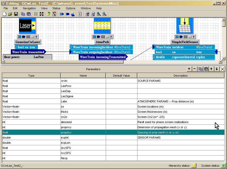
The Parameters list contains all the top-level module parameter and input symbolic names whose numerical values still need to be defined. At the top of this list panel are several buttons, of which the key ones for present purposes are the "" and "¯" buttons. To modify the list order, select (left-click) a line in the Parameters list,and then click an arrow button to move the selected line up or down an arbitrary number of places in the list. When the modified system is saved, and the corresponding Run Set is updated, the revised ordering of system variables will appear in the Run Set Editor. Note that the System Parameters list in the Run Set Editor is completely identical to the Parameters list that appears when "View -- Parameters" is selected in the System Editor. However, the parameter ordering can only be modified in the System Editor window.
(2) The second mechanism by which desired ordering can be achieved is to define auxiliary Run Variables in the Run Set Editor. As noted before, all Run Variables are considered "above" all System Parameters, therefore any existing System Parameter can be defined in terms of some new variable by creating that new variable as a Run Variable. To creating a new Run Variable, select an existing line in the Run Variables panel, and then using the "+" button in the Run Set Editor's toolbar to insert a new line at the selected location. The Run Variables panel also has "" and "¯" buttons to allow desired reordering in that panel.
Making StopTime a run variable
Near the top right of the Run Set Editor (TRE) window, we find an entry field for the simulation Stop Time. We can enter a numerical value in this field, but alternatively it could be more convenient to define the Stop Time in terms of other variables, such the desired number of sensor exposures and the exposure interval. It is not allowed to enter a formula directly in the Stop Time field. Instead, one must define a run variable, called stopTime, and assign the desired formula to that variable. The RunSet excerpt below shows an example:
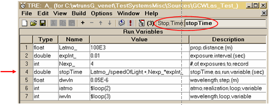
The key points are:
(1) Enter the variable name stopTime
in the Stop Time field, instead of a number. Due to some special code
restrictions, stopTime
should be the exact name used.
(2) Create a run variable called stopTime,
of type double (see
the line marked by the red arrow).
(3) Define the value of the stopTime run variable as desired in terms of
other variables. Remember to observe the restrictions on
order of definition of variables.
Importing a run set
Suppose that we create a new WaveTrain system by making just a few modifications to an existing system, and then using the menu "File -- Save As" to save under a new name. To use the new system, we must create a new runset associated with the new system. When we create the new runset, it necessary starts out with all blank Value fields in the Run Set Editor (TRE). For a complex system with many system parameters and run variables, it would be a tedious job to reenter all the setting expressions in the Run Set Editor (TRE), most of which will be identical to the old run set. To avoid this tedium, an old Run Set associated with the old system can be imported into the new runset. Once the new (blank) runset is created for the new system, we can select the menu option "File -- Import" in the Run Set Editor (TRE) window. This presents us with a subsidiary file selection window: in that window, we navigate to the old run set location, select and open it. This action imports the setting expressions for all those system parameters and run variables that have identical names in the old and new runsets. To complete the new run set, only the Value fields of entirely new variables need to be filled in from scratch.
"Add Note" feature
The System Editor has a useful documentation feature that allows the user to add a box of arbitrary text in the editor window. A so-called "Note" box is created by either (1) left-clicking on blank space, then selecting "Add Note", or (2) pulling down the Edit menu, then selecting "Add Note". This action opens a Notes Dialog box into which the user can type arbitrary text to help document the system. The dialog box can be reshaped (before closing) by grabbing its edges with the mouse. After closing the dialog box, the resulting box can be selected (left-click) in the Editor window and moved at will. To edit an existing box, right-click the box and select Edit. Additionally, right-clicking an existing box presents a few rudimentary formatting options.
In the introductory section on assembling WaveTrain systems, we mentioned that the icons that appear upon insertion of a WaveTrain library component may have several deficiencies. In one way or another, the icon may present a misleading picture of the component's function; in other cases, there is no icon at all assigned in the library. In the latter case, a small gray square appears instead of a picture. The icons can easily be customized in two ways. The key point to remember is that the icon associated with a system component has no effect whatsoever on the simulation function of the component. The picture of HartmannWfsDft could be replaced with a banana and the system would still function just fine.
The first customization option is to use a variety of alternate icons available from a WaveTrain icon library. To access these, simply right-click in the System Editor on an existing component icon (or grey square), and select the option "Edit icon". Select the radio button "All" in the resulting window that pops up, and you will see a catalog of available icons. Browse and select a desired icon, and press OK to accept your new choice.
You can also provide your own image file for use as a component icon. After you perform (right-click)-(Edit icon), simply specify your image file directory in the "Look in" box of the pop-up window, and select your own icon file. This option is useful for presentation purposes particularly when you construct user-defined composite or atomic subsystems in your WaveTrain model. Most of the WaveTrain library icons are 64x64-pixel gif images, but other sizes and file types are also accepted.
Inspecting and post-processing WaveTrain output: *.trf files, TrfView, and Matlab
WaveTrain simulation output consists of data that the user has
selected for recording in the
Recorded Outputs menu of the Run Set
Editor (TRE) When the Execute button is pressed in the Run Set Editor (TRE), the
WaveTrain simulation executes and runs to completion, but no output is automatically
displayed. WaveTrain's outputs from a given execution are stored in a specially-formatted file
that carries the extension ".trf " (pronounced "turf" by
initiates). To display and post-process Wavetrain output,
the user has two starting choices:
(1) Use the TrfView inspection and plotting utility,
launched from the Run Set Editor (TRE)
(2) Open a Matlab session, load trf-file
contents, and plot and post-process using the full power of Matlab.
Method (1), use of TrfView: This method is much easier to start with, and is the recommended starting method for all new WaveTrain users. Even more experienced users, who learned Method (2) before the existence of TrfView, will benefit from TrfView because of its ease of use and quickness to generate plots and inspect data. The restriction in TrfView is that one cannot perform arbitrary post-processing within its confines. For arbitrary post-processing, users must still import data into Matlab or another scientific computation/visualization package of their choice.
Method (2), loading of WaveTrain output data into Matlab:
(2a) Exporting from TrfView: TrfView has an export capability, which allows data to be
quickly loaded and inspected within TrfView, and then
exported to a Matlab command window for arbitrary manipulations with the full
power of Matlab. (TrfView also supports export to other destinations such as Microsoft
Excel or plain ASCII files.)
(2b) Direct loading of trf data into Matlab:
In the remainder of this chapter, we discuss
(1) The trf file naming convention
(2) The grouping of trf data by "run index (run
number)"
(3) The usage of TrfView, including its export features
(4) The Matlab functions needed to import trf data
directly into Matlab, without TrfView
All WaveTrain users should understand items (1)-(3). Regular users will eventually
want to progress to item (4) as well.
trf file naming convention
In the System Editor window, a WaveTrain system is saved under a
System Name. Likewise, in the Run Set Editor (TRE), the user saves
specifications under a Run Set Name. The recorded output data is stored in
a ".trf" file named according to the following pattern:
"SystemNameRunRunSetNameK.trf", where
SystemName
= name of the WaveTrain system (user-specified)
RunSetName
= name of the run set (user-specified)
K =
sequential numerical index automatically assigned by WaveTrain (1 higher than
previous highest index found in current directory for SystemNameRunRunSetName)
trf
= extension designating a specially-formatted data file
(pronounced "turf" by
WaveTrain initiates).
Further remarks on
K: each time a given Run Set name is executed, (usually with some modification in parameter values or system specification), a new trf file is generated. The name of the trf file is identical except for the sequentially-increasing K value, which is assigned automatically by the program.Caution on size of trf files
Since much of the interesting data in a WaveTrain simulation consists of 2-D images, it is easy to generate very large trf files (say hundreds of megabytes or several gigabytes). Using commands to be discussed below, it is possible to restrict the loading of trf data into Matlab to only selected variables or time subsets from a trf file. However, prior to actually loading data, the trf file must be opened, and the Matlab interface functions impose a limit on the size of the file that can even be opened. This limit may depend on the version of Matlab being used or some local machine installation factors. If the size of the trf file approaches 2 GB, difficulties can be expected in opening the file.
Another size issue that the user should recognize is that trf files store floating-point image-type data in single precision. However, when such data is loaded into Matlab, it becomes double precision, hence further ballooning the memory requirements.
Grouping of trf data by "run index"
Whether one uses only TrfView, or the Matlab interface, there is one aspect of the trf data grouping that must be clearly understood. This key point is the definition of a "run", and the meaning of the term "run index" or equivalently "run number".
We sometimes use the term "run" in a generic sense to indicate the overall execution of a WaveTrain simulation, but in connection with trf files we use the term "run" in a specialized sense. The specialized meaning of "run", which will be implied in our entire discussion of WaveTrain output data, is as follows: one run denotes that subset of outputs associated with one set of values of the loop variables that have been defined in the run set.
Example 1: A run set might have no loop variables. That is, each input parameter defined in the Run Variables panel of the Run Set Editor (TRE) has one and only one value. In that case, the output trf file generated when "execute" is pressed in the Run Set Editor will contain output data for one "run", whose run index is 1. RECALL that this single "run" might contain output data for each of many time steps: the sample times specified in WaveTrain's sensor specifications do NOT correspond to a loop index in the present sense.
Example 2: In general, the specifications in the Run Set Editor (TRE) may include one or more loop variables. That is, WaveTrain executes the simulation once for each combination of loop variable values, and the output for each combination is called a "run". For example, suppose there are two loop variables, with the first cycling through two values, and the second cycling through three values: in that case, there will be 2x3 = 6 "runs", designated by a one-dimensional "run index" whose values are 1,2,...,6. Data from all six "runs" will be stored in the single trf file generated by the WaveTrain execution of this Run Set.
The order mapping from the {2 x 3} space to the
one-dimensional run index is
illustrated in the explicit example below:
Excerpt from a WaveTrain run set
First, we are interested in the Run Variables panel of this runset (eventually, we will come back to the Output Recording snapshot at right). We have defined two loop variables, called iatmo and iwvln, which will take on two and three values, respectively, during the execution of the run set. For purposes of the trf-file organization, WaveTrain combines the two loop indices into a one-dimensional "run index" according to the following rules:
(1) The order
in which the loop variables appear in the runset defines a nested execution
order for the run set, as defined by the following pseudo-code:
for iatmo = 0 to 1
for iwvln = 0 to 2
...
end; iwvln loop
end; iatmo loop
(2) As indicated in (1), loop indices start with the value 0, in accordance with C-language indexing conventions (the visual editor actually converts a run set into C++ code).
(3) The one-dimensional run index is a sequential counter that starts at 1, and is incremented by one whenever any loop index is incremented in the nested sequence defined by (1). Thus, in the case of the above two loop variables, the association between loop indices and run index is illustrated in the following table:
| iatmo | iwvln | run index |
|---|---|---|
| 0 | 0 | 1 |
| 0 | 1 | 2 |
| 0 | 2 | 3 |
| 1 | 0 | 4 |
| 1 | 1 | 5 |
| 1 | 2 | 6 |
Any number of loop variables is allowed, in which case the nesting in (1) extends in the obvious way. It is not unusual for a WaveTrain runset to have only one or even no loop variables. If there are no loop variables, the WaveTrain run index spans only one value, namely 1.
Given an understanding of the above run index concept, the usage of TrfView to inspect WaveTrain output is fairly intuitive. To start TrfView, open a run set in the Run Set Editor (TRE) window, and press the TrfView button circled in the following figure:
Pressing this button opens the chronologically latest trf file associated with the run set, and presents the main TrfView window, as illustrated below:
(Once the main TrfView window is open, its File menu may be used to open other trf files, including ones belonging to completely different run sets. However, only one run set can be open at a time in TrfView).
The main TrfView window displays four columns.
Column 1 lists all the variable names that were saved in the trf file.
These are the variables that were checked
for recording in the Run Set Editor prior to execution of the WaveTrain run.
Column 2 lists the data type of the scalar elements of each recorded
variable (i.e., an array of floats is just designated "float").
Column 3 lists the number of time steps at which values of each variable have
been recorded.
Column 4 lists dimensional information: (a) if the variable is 2-D
image-type data; then "(NX)x(NY)" gives the pixel dimensions of the 2-D images;
(b) if the variable is not a 2-D image, it may represent a single scalar or a
vector, whose dimensions are listed as (N)x(1).
The following caution applies to WaveTrain
versions 2009A or earlier:
CAUTION:
Actually, column 4 only lists the probable space dimensions
of each data variable. The "probable" qualifier obviously requires some
explanation. Consider a multi-dimensional data variable such as the
irradiance array I(ix, iy, it), where (ix, iy) are spatial indices and (it) is
the time index. Let (nx, ny, nt) be the physical dimensions of the
recorded data. For historical reasons, such an array is actually recorded
in the trf file as a 2-D array, of dimensions (m=nx*ny, nt).
Unfortunately, the trf file does not automatically record the values of
nx and ny, so there is no foolproof automated method of reshaping the (m)
values for plot purposes. TrfView makes a reasonable guess at (nx,ny), and
these are the values that are first reported in Column 4. The guess is
formulated as follows:
(a) If sqrt(m) is an integer, TrfView reports that (nx, ny) = (sqrt(m), sqrt(m)).
(b) If sqrt(m) is not an integer, TrfView reports that (nx, ny) = (m, 1).
This guess is the most reasonable one, because square sensor arrays are the most
common configuration, but of course that will sometimes be wrong. If the
spatial data is not square, the user must manually tell TrfView what the
correct dimensions are by pressing the "..." button at the right of column 4 and
entering the correct dimensions. Note that in Wavetrain, "x"
Selecting runs within a run set
In the main TrfView window illustrated above, note the tool bar located just below the menu bar. The item "Runs in File: 1" in the illustration indicates that this run set and trf file contain one "run" in the specialized WaveTrain sense explained earlier in this chapter. If there had been more than one run in the trf file, then the adjacent list "Select Run" could be pulled down to select any desired run number within the trf file. All the variable listings in columns 1-4 would stay the same, but the data values would of course usually change if we change run number.
Plotting and inspecting the data in TrfView
TrfView provides good quick-plot and data-inspection capabilities, and a limited number of post-processing options. To perform custom plotting, add arbitrary plot annotations, or do arbitrary post-processing, the user must either export the data from TrfView to Matlab, or load the trf data directly into Matlab: those procedures are explained in subsequent sections.
The menus and options for
plotting within TrfView are fairly self-explanatory. To briefly
illustrate, let us return to the previous
figure showing a TrfView main window. Suppose we want to plot the
variable named "... pt_diag_cam.fpaImage" (5th name in the variable list, which
happens to be highlighted in the figure). From knowledge of the WaveTrain
system, this variable happens to corresponds to the
integrated intensity map seen by a camera
sensor. Column 4 of the TrfView window shows the spatial dimensions of
this data to be 256x256. To plot the integrated intensity map, we
can either
(a) left-click on the variable to select it, then use the menu command "Variable
- Plot Variable"; or,
(b) right-click the variable name, and select "Plot Variable".
This causes TrfView to generate a separate plot window as illustrated in panel
(A) of the following figure:
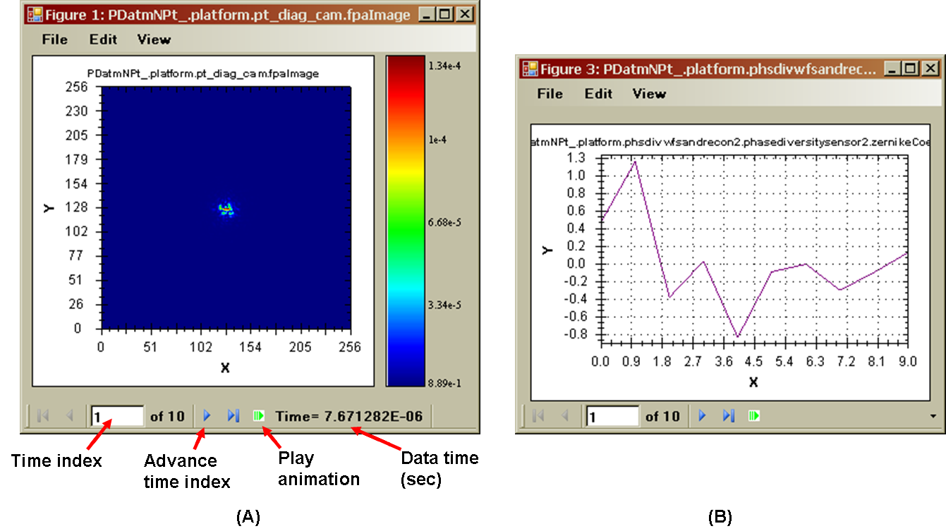
Below the plot itself, the plot window in panel (A) has a time index entry field: by entering a different index number, or clicking on the neighboring arrow buttons, we can see the 2-D map at any of the recorded times. The actual simulation time, in seconds, to which the data corresponds, is also listed. (Recall that column 3 of the main TrfView window also specified how many time steps were recorded.) The plot window also has button (see panel(A)) that plays an animation of the full time-sequence of 2-D maps. The color bar has a numerical scale that quantifies the map values.
In the case of a vector variable,
TrfView plots a line-plot of the vector elements versus element index.
Consider the variable named "... zernikeCoeffs" in our example TrfView
window (3rd variable in the list). At
any time index, this particular 10x1 vector happens to contain the values of
Zernike expansion coefficients that were used to represent a wavefront.
Applying the plot command on that variable yields the plot shown in panel (B) of
the above figure.
Note 1: Vector element indices span 0,1,...,N-1 in accord with
C/C++ conventions, hence the data point locations in panel (B).
Note 2: As we see in panel (B), the default axis scales created by
TrfView for line plots are often somewhat inconvenient. In panel (B), it
would obviously be preferable to have scale number 0,1,...,9 or 10. The
user can adjust the axis scale values to some extent by right-clicking on
the plot, and selecting the option "Set scale to default". In the present
example, that produces nicer scale numbers.
Note 3: As we see in panel (B), the horizontal and vertical axes of
a line plot are always labeled "X" and "Y", even though these axes typically
have nothing to do with spatial directions.
Other plot-view options:
other useful font and graph display options can be accessed by
(a) right-clicking on the plot to bring up a context menu
(b) pulling down the "View" menu in the plot figure window.
Note that the options provided under (a) and (b) are not the same.
Zooming: To magnify (zoom in on) a section of a plot, we can left-click and drag to outline the section that we want to magnify. To undo the zoom, we right-click in the plot and select "Unzoom".
There is another plot-control window also generated by TrfView as soon as the first plot is created. This window is illustrated in the following figure, after we have created two plot windows (the ones in panels (A) and (B) above):
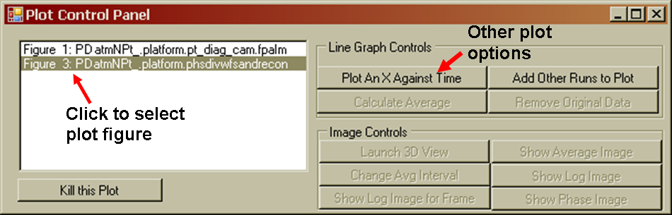
This control window contains a listing of all the plot figures currently open, and the user can select any figure in the list by left-clicking it. Depending on the nature of the selected plot (line or image), a number of other plot (or analysis) options then become available on the right side of the window. Perhaps the most useful of these is the line-plot button that says "Plot an X against time": in connection with the previous panel (B) example, pressing this button allows the creation of a line plot of one of the Zernike coefficient values versus the time index.
Inspecting data numerical
values: if we want to do better than visually reading off the plot
scales, TrfView provides several options:
(a) In an image or line plot: the menu command "View - Data" toggles on
and off a small sub-window that displays the array or vector numerical values.
(b) In a line plot such as panel (B): right-clicking on the plot brings up a
context menu that contains the option "Show point values": after that
option is selected, hovering with the cursor over a data point causes that
point's coordinate values to appear.
Archiving (saving) plots
Usually, one wants to save some
plotted results in a presentation (e.g. PowerPoint) or word-processing file.
TrfView provides several options for saving plots, among which are:
(a) In a TrfView plot window, use the menu command "Edit - Copy to
clipboard" to copy the window to the Windows clipboard. (This is the same
as using Windows' traditional "Alt-PrtScrn").
(b) Right-click on a TrfView plot, select "Save figure as ...".
(c) In a TrfView plot window, use the menu command "File - Export to
...". For example, one option is to export to PowerPoint: this has
the effect of adding a new slide to a user-designated PowerPoint file, and
copying the plot to that slide.
Another TrfView archiving option is the automatic creation of an AVI movie file. This feature is accessed through the menu sequence "File - Export To - AVI file" in a TrfView plot window.
Exporting data from TrfView to Matlab (or other analysis environments)
As noted previously, TrfView does not provide arbitrary plot customization or post-processing analysis. To accomplish such tasks, we must either (a) export the trf data from TrfView to Matlab (or other analysis environment), or (b) bypass TrfView completely and read trf data directly from Matlab. We discuss option (b) later in this chapter.
Exporting data from TrfView to
Matlab is very simple. Consider again the TrfView main window figure
illustrated earlier. To export the
data for variable "... fpaImage", we can either
(a) left-click on the variable to select it, then use the menu command "Variable
- Send to Matlab workspace"; or,
(b) right-click the variable name, and select "Send to Matlab workspace".
Assuming that we have a working installation of Matlab on the same computer, and WaveTrain's environment settings have been told the Matlab path, actions (a) or (b) will cause a Matlab command session to open, and will cause a Matlab variable corresponding to "... fpaImage" to appear in that session. The following figure is a screen capture of the Matlab command window, after we have added a few Matlab commands.
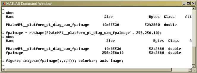
In the above Matlab window, the
sequence of events and their motivation was as follows.
(1) Immediately after we issued the data export command in TrfView, the
Matlab command window opened blank.
(2) We entered the first Matlab command,
>> whos
Matlab reports that a variable named "PDatmNPt__platform_pt_diag_cam_fpaImage"
is present in Matlab's workspace: this is the data exported by TrfView.
Furthermore, Matlab reports the dimensions of the variable to be 10x65536.
Back in the TrfView main window, the variable data was designated as having 10
time steps, with (x,y) dimensions of 256x256. Note that 2562 =
65536. This explains the dimensions 10x65536 of the Matlab variable.
Note that all 10 recorded images, one for each time step, have been imported
into a single Matlab array variable.
(3) For subsequent processing, it is an inconvenience that the variable
was imported as 10x65536, rather than the more natural 256x256x10. This
has to do with the early history of WaveTrain and trf files. It is almost
always more convenient to reshape the array data to the natural 256x256x10
dimensions. We accomplish this with the next Matlab command,
>> fpaImage =
reshape(PDatmNPt__platform_pt_diag_cam_fpaImage', 256,256,10);
Notice that the original variable is transposed (using the ' operator) before
the reshape is actually applied. Users of Matlab will understand this
command syntax. Another
>> whos
command confirms the desired shape of the renamed variable.
(4) At this point, the data is in convenient form for arbitrary Matlab
plotting or processing. For example, the last command in the window,
>> figure; imagesc(fpaImage(:,:,1)); ...
generates a Matlab plot of the image for time index 1.
Exporting to other analysis or display environments:
TrfView supports the export of trf data to the Microsoft Excel spreadsheet program, and to CSV (comma-separated values) text files. These export features are accessed from a TrfView plot window, by using the menu sequence "File - Export To...". The resulting listing presents the currently-supported export destinations. Note that the Excel program allows a maximum of 65536 rows, but only 256 columns: this limits the array size that can exported from TrfView.
In general, importing Wavetrain results into analysis environments other than Matlab is not as well supported as the Matlab interface. Specifically, the WaveTrain suite does not provide read routines for direct import of trf-file data into environments other than Matlab.
Parameters tab
The above discussion of TrfView has all been related to the tab labelled "Variables" in the main TrfView window. Inspection of the window also shows a second tab, called "Parameters". The "Variables" tab referred to outputs that the user requested WaveTrain to record, by selecting variable names for recording in the Output Recording menu of the Run Set Editor (TRE). On the other hand, the "Parameters" tab contains auxiliary information that was recorded by WaveTrain by default in the trf file. This auxiliary information comprises the values of the Run Variables and System Parameters that were specified in the Run Set Editor (TRE) prior to execution. This information is not needed for TrfView plotting purposes, but obviously constitutes valuable documentation of the parameter settings used for the Wavetrain runs contained in the trf file.
Loading trf data into Matlab without TrfView
As explained in the
introduction of this chapter, the most general and powerful way of
post-processing WaveTrain's trf-file output is to directly import trf
data into the Matlab analysis and visualization environment. WaveTrain
provides complete support for this procedure, via a number of read functions
that are to be used at the Matlab command prompt. Usage of the functions
is fairly straightforward, and requires the following:
(a) a basic understanding of Matlab syntax;
(b) understanding of the trf data structure as imported into Matlab;
(c) understanding of a small number of file-open and file-load commands
that must be executed at the Matlab command prompt.
Items (b) and (c) are explained in the remaining sections of the present
chapter.
All output data from the execution of a WaveTrain run set is collected into a single data structure, whose fields correspond to the individual runs of a run set and to the individual variables (scalars, vectors, or arrays) that were ticked for recording.
Fields of the trf data structure
Suppose that we read the entire
trf data structure into Matlab (using commands
to be explained below), and that we assign it the name ds. The
entity ds is a data structure in the sense that Matlab uses that term,
and we assume that the reader knows the basic syntax rules for manipulating
Matlab structures. Only the basics are really necessary for working with
the trf-derived data. The key point is that the simulation's
physical output data is contained in the two structure fields
ds.r(irun).v(ivar).d:
temporal sequence of recorded data entities
ds.r(irun).v(ivar).t:
sequence of sample times corresponding to the data sequence d.
The index irun is any
value of the run index defined above, and ivar
is any value of an index that specifies which recorded variable is in question.
The trf-commands section below shows how to
determine the mapping between recorded variable names and
ivar
values.
The sequence of sample times is determined by the exposure specifications in the WaveTrain system's sensor modules. The sample time always corresponds to the end of a sensor exposure length window. The data entity ds.r(irun).v(ivar).t is a row vector in Matlab.
The composition of the data
entity ds.r(irun).v(ivar).d
depends on whether the recorded variable is a scalar, a vector or an array.
Suppose the recorded variable is a:
(1) Scalar : for example, the recorded variable may be the peak
pixel intensity in a image. In this case, there must be one recorded
number for every sample time, and the entity d
is a vector of the same length as the t
vector.
(2) Vector : for example, the recorded variable may be encircled
energy ("energy-in-bucket") versus circle radius. In this case, there must
be one recorded vector for every sample time. The entity
d encodes this as a 2-D array
of the form d(ir,it),
where the first index, ir,
corresponds to the different circle radii, and the second index,
it, is a time index that
corresponds to t.
(3) Array : for example, the recorded variable may be the
integrated intensity (J/m2) of a two-dimensional image. In this
case, there must be one recorded 2-D array for every sample time. The
entity d encodes this
as a 2-D array of the form d(ip,it),
where the first index, ip,
corresponds to all the pixels in the image, and the second index,
it, is a time index that
corresponds to t.
Since the d entity
uses a single index, ip,
to index the pixels of a 2-D image, the user must use Matlab's "reshape"
function to obtain 2-D indexed images for display or further processing.
The pixels of the 2-D image contained in
d(1:Npix, fixed it)
are ordered with x-coordinate index varying most rapidly.
Some usage examples that illustrate the above trf-data formats are given in the following section devoted to key trf commands.
Key commands for working with trf data in Matlab
In this section, we cover the key
commands that can be used at the Matlab command line to load trf data
structures, to extract data for desired runs and variables, and to obtain
information about the trf contents. We discuss the following list of six
basic functions:
trfopen
trfrlist
trfvlist
trfload
trfclose
tmxparams.
For advanced trf-file users and programmers,
additional commands and general
information are available in separate documents; however, most WaveTrain
users will be able to go a long way using the six basic functions discussed
here.
The examples below are all based on a trf file generated by the run set excerpt pictured previously. The name of the trf file is "GCWLas_Test_RunA_3.trf". The function usage examples are ordered so as to take the reader through a logical sequence of commands to open a trf file, inspect critical indexing information, and then load and manipulate desired physical data. In the examples below, the symbol ">>" denotes the Matlab command prompt.
trfopen
Prior to loading any trf data, we must open the file. At the Matlab prompt, we enter:
>> th = trfopen('GCWLas_Test_RunA_3.trf')
The function responds with:
th =
filename: 'GCWLas_Test_RunA_2.trf'
fid: 4
machineformat: 'ieee-le.l64'
addresstype: 'int64'
parameters: []
r: [1x6 struct]
The symbol th is a user-specified name that constitutes a "trf handle". The function response is mostly uninteresting to the user, except for the last line which indicates that the data structure run field, r, is a 1x6 structure. This tells us that the trf file contains 6 runs, corresponding to the values 1 to 6 of the run index defined by our run set excerpt. The function response can be suppressed by the standard Matlab procedure of terminating the command line with a semi-colon. Notice that th is itself a Matlab structure.
trfrlist
The trf handle contains much useful information about the file contents, and it is often useful to inspect this information prior to actually loading any simulation output data. The first useful inspection function, trfrlist, can be used to remind us of the mapping between the loop variables and the run index. At the Matlab prompt, let us enter:
>> trfrlist(th)
The function responds with:
ans =
1 - iatmo=0,iwvln=0
2 - iatmo=0,iwvln=1
3 - iatmo=0,iwvln=2
4 - iatmo=1,iwvln=0
5 - iatmo=1,iwvln=1
6 - iatmo=1,iwvln=2
This is exactly the mapping that was defined in the example table that accompanied our earlier definition of "run index".
The second critical inspection function, trfvlist, is used to remind us what output variables were recorded in the trf file, and to tell us the mapping between the variable names and numerical indices. The numerical index is needed when we want to extract specific data from the composite data structure. At the Matlab prompt, let us enter:
>> trfvlist(th.r(1))
The function responds with:
ans =
1 - A_.irradprobe.intgr_intens
2 - A_.simplefieldsensor.fld
3 - A_.targetboard.integrated_intensity
The numbers in the first column of the output are the variable numerical indices that have been assigned by WaveTrain. The names after the dashes begin with the run set name ("A_", in this case) followed by the subsystem and variable names. We see that these names are identical to the names that were ticked for recording in the Output Recording menu of the run set excerpt pictured earlier.
If a variable named "integrated_intensity" were buried three layers down in a hierarchy of subsystems, its full name as reported by trfvlist might be "RunSetName.level1sys.level2sys.level3sys.integrated_intensity". The ordering of the variables is alphabetic, by hierarchy level.
The responses to trfvlist(th.r(2)), etc., are identical to the run 1 case, because all the runs have the same recorded variables.
trfload
After exercising the trfrlist and trfvlist functions, we know all the numerical indices needed to extract and work with specific data of interest. Let us now load some of the simulation output data into Matlab, using the trfload function, and then begin to manipulate the data.
Example 1: Loading the
entire trf-file contents into Matlab.
At the Matlab prompt, we enter:
>> ds = trfload(th)
The function responds with:
ds =
filename: 'GCWLas_Test_RunA_3.trf'
fid: 5
machineformat: 'ieee-le.l64'
addresstype: 'int64'
r: [1x6 struct]
The symbol ds is a user-specified name for the Matlab data structure that now contains the entire trf-file data set. Following the standard Matlab command syntax, the function response can be suppressed by terminating the command line with a semi-colon.
Recall now the introductory
discussion of the fields of the
trf data structure. Suppose that we are interested in the data
from run index 2 (i.e., iatmo=0 and iwvln=1). Suppose further that we want
to extract into new workspace variables and further process the simulation
output data corresponding to the variable
A_.targetboard.integrated_intensity. According
to the output of trfvlist,
the variable of interest has numerical index 3. As noted in the previous
discussion of the fields of the
trf data structure, we are primarily interested in the structure fields
ds.r(2).v(3).t
and
ds.r(2).v(3).d
Before extracting these data into new variables, let us inspect the format of the t and d entities. We can do this in one operation, as follows:
>> ds.r(2).v(3)
Matlab responds with:
ans =
varname: 'A_.targetboard.integrated_intensity'
varnumber: 3
anextvars: 0
anextdb: 939507
id: 3
typename: 'A_.targetboard.integrated_intensity'
description: 'Integrated intensity'
flags: 6
type: 3
nobjs: 16384
t: [0.0013336
0.011334 0.021334 0.031334]
d: [16384x4
double]
The first line of the response is useful as confirmation that we have indeed specified the desired variable.
The only other lines of interest are the last two, which give us the dimensions of the physical data arrays of interest. From the ds.r(2).v(3).t specifications, we see that a temporal sequence of four output entities has been recorded, corresponding to the four sensor exposures that were set up in the run set. As noted previously, the sample times correspond to the end of the specified sensor exposure length windows. In the present case, because there are only four elements in the t vector, the values are printed in the above response. Usually, the format of the response would be "t: [1 x Nt double]", where Nt is the number of sample times.
The final entity of interest is of course ds.r(2).v(3).d. This contains the numerical values of integrated_intensity at all the sample times. As discussed previously, the format of the d array is d(1:Npix, Nt), where the first index spans all the pixels in one 2-D image, ordered with x-coordinate varying most rapidly. For most (but not all) purposes, it is much more convenient to reshape image data so that x and y pixels have separate indices.
Prior to reshaping and further processing, it may be convenient (though not necessary) to extract the time and image data into new variables, perhaps with more meaningful names. For example, let us continue by defining two new Matlab variables:
>> t =
ds.r(2).v(3).t;
>> ii = ds.r(2).v(3).d;
Note that here we almost always
want to terminate the Matlab command lines with the semi-colon, otherwise Matlab
will flood the screen with the array values.
Now let us continue by using Matlab's "reshape" function to reshape the existing
ii array into a more
convenient form, with final dimensions 128x128x4 (since 128^2=16384):
>> ii = reshape(ii, 128,128,4);
At this stage, ii is a 3-D array with dimensions (128,128,4), where the first dimension corresponds to the WaveTrain x-index, the second corresponds to the WaveTrain y-index, and the third corresponds to the time dimension. At this stage, t and ii are in convenient form for any further image display or processing manipulations that the user cares to perform using any of the standard Matlab machinery.
When reshaping is done, the user must know (from familiarity with the WaveTrain system) what the x and y dimensions corresponding to 1:Npix are. In practice, a recorded image array is usually square, but this is not a necessary condition. If Nx and Ny are defined as run variables or system parameters, then the numerical values are encoded in the trf file, and the user can obtain them by exercising the tmxparams function; otherwise, the user must know the values from familiarity with the WaveTrain system.
Additional recorded data, as of WaveTrain ver.
2010A:
An item that was lacking in previous WaveTrain versions was the recording of
mesh coordinate information for recorded Grid
variables. Recall that a Grid in the specialized WaveTrain sense
consists of an x-y mesh of points, together with values of some function on that
mesh (e.g., a 2-D irradiance map). Previously, only the function values on
the mesh were recorded, in the
The new feature in WaveTrain
2010A is that mesh coordinate vectors are automatically recorded in the
trf file whenever a Grid variable is recorded. This is done by
creating two additional variables names with auto-generated names. For
instance, consider the recorded-variables listing produced above by the
trfvlist command: variable number 3 was
A_.targetboard.integrated_intensity
These are the integrated-intensity values of a 2-D integrated-intensity
map. As of WaveTrain version 2010A, for every such Grid variable, there
will also appear two auxiliary variables with auto-generated names:
A_.targetboard.integrated_intensity_xauto
A_.targetboard.integrated_intensity_yauto
These two auto-generated auxiliary variables are
vectors that contain, respectively, the x- and y-coordinate values of the mesh
on which targetboard.integrated_intensity
(or whatever other name) exists.
The new feature will be helpful for post-processing.
Example 2: Loading
partial contents of a trf-file into Matlab (run, variable restriction)
Because of memory capacity, it is often not practical or desirable to load an
entire trf file into Matlab. The trfload
command has several useful options in this regard. The general syntax of
trfload, with optional
arguments indicated by { }, is as follows:
>> ds =
trfload(trfhandle,{runs},{variables},{mintime},{maxtime})
where runs
is a vector of run indices
variables is a vector of
variable indices
mintime and
maxtime are each a scalar time limit (in units of
seconds).
For example, suppose we want to load only runs 2 and 4, and only variables 1 and 3 from the same trf file used in Example 1. At the Matlab prompt, let us enter:
>> dsB = trfload(th, [2 4], [1 3])
The function responds with:
dsB =
filename:
'GCWLas_Test_RunA_3.trf'
fid: 6
machineformat: 'ieee-le.l64'
addresstype: 'int64'
r: [1x2 struct]
Note that the run entity,
r, is now only 1x2,
indicating that only two specified runs have been loaded.
CAUTION: Although the specified runs were indexed by 2 and 4 in the
trf file, they are indexed by 1 and 2 after loading into the Matlab
structure variable
dsB. In fact, if we
exercise the trfrlist
function on dsB:
>> trfrlist(dsB)
then the function returns:
ans =
1 - iatmo=0,iwvln=1
2 - iatmo=1,iwvln=0
If we exercise the function trfvlist on dsB, we find:
>> trfvlist(dsB)
ans =
1 - A_.irradprobe.intgr_intens
2 - A_.targetboard.integrated_intensity
Comparing this with the previous
output of trfvlist, we
see that indeed only the original variables indexed 1 and 3 have been loaded.
CAUTION: Although the specified variables were indexed by 1 and 3
in the
trf file, they are indexed by 1 and 2 after loading into the Matlab
structure variable dsB,
as indicated by the preceding trfvlist
output.
CAUTION: Note that in the immediately preceding usages of trfrlist and trfvlist we have used the data structure dsB as the argument, rather than the trf handle th as we did earlier. These two functions can operate on either the trf handle or the data structure. When we want the index mappings for just the restricted data set that has been loaded, we must of course use the corresponding data structure, and not the trf handle that corresponds to the entire data file.
In order to omit a preceding option in trfload, we must supply the Matlab empty variable, [], in the omitted position. Undesired trailing options can be omitted completely. For example, to load all runs but only variable 3, we would enter:
>> dsC = trfload(th, [],
[3])
For the run set in question, this is actually
equivalent to
>> dsC = trfload(th, [1 2 3 4 5 6], [3])
Example 3: Loading
partial contents of a trf-file into Matlab (time restriction)
The option of restricting loading to less than the full time length of the
recorded outputs can also be very useful. If the {mintime}
and {maxtime}
arguments are specified, in units of seconds, then all data whose sample times
fall between mintime
and maxtime,
inclusive, will be loaded. Time restriction may be combined with the run
and variable restrictions. For example, we can load data from all runs and
all variables, between specified times as follows:
>> dsD = trfload(th,[],[],0.01,0.03)
dsD =
filename: 'GCWLas_Test_RunA_3.trf'
fid: 6
machineformat: 'ieee-le.l64'
addresstype: 'int64'
r: [1x6 struct]
From the dimension of the returned r field, we see that the command has loaded data from all six runs. Then,
>> dsD.r(1).v(3)
ans =
varname:
'A_.targetboard.integrated_intensity'
varnumber: 3
anextvars: 0
anextdb: 136157
id: 3
typename: 'A_.targetboard.integrated_intensity'
description: 'Integrated intensity'
flags: 6
type: 3
nobjs: 16384
t:
[0.011334 0.021334]
d:
[16384x2 double]
shows that data for only those sample times between 0.01 and 0.03 has been loaded (compare with the original four sample times loaded when time was unrestricted).
trfclose
When a data file is no longer needed, it is recommended to explicitly close the file, using:
>> trfclose(th)
where th is the trf handle that was assigned upon opening the file.
The trf file documents the numerical values of all run variables and system parameters defined in the run set. This can very useful, particularly when writing post-processing m-files or scripts whose computations depends on some parameters values: the script code can then be written in terms of a variable parameter value, and the actual value can be extracted from the trf file. The function tmxparams returns all the run variable and parameter values, as follows:
>> tmxparams(th.r(1))
ans =
GLasDap: 0.3
GLasPow: 10
GLasSigma: 0.2
Latmo: 100000
Latmo_: 100000
Nexp: 4
Nexp_: 4
RXnxy: 128
alt: 10000
clear1Factor: 1
dwvln: 5e-008
etc ...
The above list has been truncated here for brevity. Comparing the list with the run set excerpt picture shown previously, the reader can see that the run variables in the excerpt picture form part of the tmxparams output list. The same output is produced if the data structure ds is used in the function argument, i.e., if we enter tmxparams(ds.r(1)).
CAUTION: WaveTrain's recording of parameter values is incomplete in the following sense. Values of the "run variables" and "system parameters" (those quantities that appear in the Run Set Editor (TRE) window) are recorded in the tmxparams list. However, parameter values that are numerically set in System Editor windows are not recorded in the trf file and hence are not reported by tmxparams. This fact by itself can be a good reason for "elevating" a parameter to the Run Set level.
Miscellaneous remarks
It is important to remember that some trf functions (for example trfrlist, trfvlist, tmxparams) accept either a trf handle or a data structure in their arguments. We have given several examples above, and situations when one or the other is needed.
The output of the functions
discussed above can always be assigned to a Matlab variable. For example,
it may be useful to assign:
>> vlist = trfvlist(ds.r(1));
>> plist = tmxparams(th.r(1));
The resulting Matlab structure variables can then be
manipulated in the usual Matlab ways in script and m-file processing. For
example, in the plist
structure, each subsidiary field of the structure is one of the parameters.
This approach is needed, for example, if we want to construct post-processing
code that automatically extracts a parameter value.
Creating user-defined WaveTrain components
The perfect and complete WaveTrain would contain library components that allow users to assemble any possible system they wish. Although the existing WaveTrain libraries are extensive, they do not provide everything that a user might want. However, WaveTrain is extensible in several ways, meaning that users can design and implement new types of components to meet new needs. Depending on the nature of the desired component, the design and implementation may be very quick and easy, or it may require considerable work and programming expertise.
A situation in which it is easy to create a user-defined component is the following. It often happens in the course of extended WaveTrain usage that we find ourselves repeatedly assembling a certain specific grouping of library components. A very simple example might be the concatenation of an Aperture module and a Focus module. A more complicated example might be the combination of library sensors and timing triggers to model a combined near-field/far-field irradiance probe. A third example is the decomposition of a complicated WaveTrain system into logical blocks such as transmitter, target, receiver, etc., each of which can be represented at the top system level by a single WaveTrain component. The common theme of these examples is that, for reasons of compactness and/or quick reusability, we often want to create a "composite" subsystem that can thereafter be dropped as a single unit into future WaveTrain systems. This procedure is very easy, and is almost identical to creating a top-level system model.
A different situation exists when the desired functionality cannot be obtained, or can only be inconveniently obtained, by using combinations of existing components. This may occur if we wish to model a type of source, optic, sensor, processing algorithm or atmospheric interaction process not provided in existing libraries. In these situations, we must create new "atomic" components. WaveTrain provides several mechanisms, of varying levels of difficulty, that allow the user to create custom atomic components. After the user creates such a component, it will have an interface of the same type as any WaveTrain library component, and the new atomic component can be inserted in the System Editor just like any WaveTrain library component.
Creating a new component by composing existing library modules
If the desired new WaveTrain module can be obtained using a combination of existing WaveTrain library components, the construction procedure is very simple. Some of the components in the WaveTrain library are themselves implemented in precisely this fashion. An example is the Telescope, shown below, which consists of a Focus and an Aperture, linked in series:
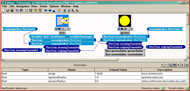
Creating these kinds of components is almost exactly like creating system models; the main difference is that components are by definition intended for use as subsystems within a larger system, and therefore they will generally have Inputs and/or Outputs, whereas a top-level system does not. (Here we are using the terms "input" and "output" in the technical WaveTrain/tempus sense.) There may also be some difference in our design approach: in designing a component meant for reusability, we want to try to foresee various circumstances under which it might be used, and tailor the functionality and interface accordingly. The main point is that we want to ensure that any parameters of the component's subsystems that the user is likely to want to change are accessible via the component's parameters. Of course, we can always go back and make changes later, if necessary, but it will result in much cleaner work if a good design is made before incorporating the new component into numerous containing systems.
To create a composite subsystem, the steps are:
(1) Open a new system window in the System Editor.
(2) Insert and connect the desired WaveTrain library components, and
assign numerical values or symbolic names in all the component parameter fields.
(The symbolic names will become parameters of the composite system.)
(3) Using the System Editor "Edit" menu (or simply right-clicking in blank
space), select "Add Input or Output". Fill in the Type, Name and Value
fields. The Telescope system illustrated above gives a syntax example.
(4) Save the composite system in exactly the same way as you would save
any WaveTrain system.
Note that step (3) is the only thing that distinguishes the creation of a composite subsystem from the creation of a top-level WaveTrain system. Note that the illustrated Telescope system has only inputs and outputs of type "WaveTrain", but in general a composite subsystem may have inputs and outputs of any data type allowed in WaveTrain.
To insert a composite subsystem into another WaveTrain
system, the steps are:
(1) In the System Editor, create or open the system into which you wish to
insert the existing composite system.
(2) Using the System Editor "Edit" menu (or right-clicking in blank
space), click "Add subsystem - Browse", navigate to the user directory where you
saved your composite subsystem, select the "YourSystem.tsd" file, and click
"Open".
The user-defined composite subsystem will now appear in the System Editor window in exactly the same way that a WaveTrain library component does. If desired, we can add a pretty icon to the subsystem by right-clicking on the blank icon block, and selecting "Edit icon".
Creating a new atomic component from a Matlab m-file (m-system)
Sometimes we may need functionality which cannot be obtained using any combination of existing components, typically because there are one or more new physical components or effects we need to model. In such cases we must define one or more new types of atomic systems, i.e. components not made up of simpler components.
For users conversant with Matlab, the following four-step procedure provides a relatively simple way of creating a new WaveTrain atomic component:
(1) Write a
Matlab m-file that has the desired functionality:
The
input arguments of the m-file will correspond to either (a) inputs that the m-file
WaveTrain component will
receive from other WaveTrain components, or (b) parameters that specify
numerical properties of the functionality.
The output arguments of the
m-file will correspond to output quantities that the m-file WaveTrain component
can pass on to
other Wavetrain components.
Note that the m-file WaveTrain component (called an "m-system") will have
"inputs", "parameters", and "outputs" just like any WaveTrain library system.
(2) Insert one
specially-formatted comment line into the m-file:
This will allow a
WaveTrain translation tool to properly define WaveTrain system inputs,
parameters and outputs for the new component. This single,
specially-formatted comment line is the only departure from standard Matlab code
that is required in constructing the m-file.
(3) In a console command
window, run the WaveTrain translation tool called msystem:
> msystem
User_mfile_name
Running the translation tool creates the file "MliUser_mfile_nameMfile.tsd",
along with a few other associated WaveTrain files.
(4) At this point, the file "MliUser_mfile_nameMfile.tsd" constitutes a WaveTrain "m-system", and can be treated essentially like any WaveTrain library component. In particular, from a WaveTrain System Editor window, the m-system can be added to a WaveTrain system in exactly the same way that we add any WaveTrain library component. When the m-system is added in this way, the usual type of WaveTrain component icon appears, with its input and output connector bars and its list of parameters.
Details of the specially-formatted comment line, and some examples, are given in a linked document.
CAUTION 1: a potentially tricky point in using an m-system is the triggering of the system. WaveTrain use a certain event-driving logic that forces subsystems to compute only when their outputs are required by some downstream system (the concept of "lazy evaluation"). Depending on how an m-system interacts with the WaveTrain library components to which it is connected, this lazy evaluation strategy can sometimes result in the m-system remaining inactive for no reason that is obvious to the user. As part of testing a system that contains an m-system, the user should record sufficient test variables to ensure that the m-system is actually being triggered (testing a couple of time steps at the beginning of a run will be sufficient). A good way of guaranteeing that an m-system is triggered is to create an input for it which is attached to a SquareWave. In that case, every transition (0®1 and 1®0) of the square wave constitutes an input change that by default triggers the m-system to compute a new output. (The input variable that represents the square wave level need not be used for anything by the m-system code: the triggering is related to the issue of the m-file being called at all).
CAUTION 2: a simple but easily overlooked
trouble spot when using m-systems concerns the Matlab path. As discussed
in the
linked document, an m-system is created that
defines the interface used by WaveTrain to mesh this new component with other
WaveTrain components. However, the computational code is still contained
only in the m-file. During actual execution of the simulation, when
WaveTrain needs to use the m-file code, it opens a new Matlab command window and
runs the m-file in that window. Now the potential trouble spot is that the
user's m-file must be in the Matlab path. One way of ensuring this is to:
(a) put the m-file in the same directory as the WaveTrain system, and
(b) add that directory to the Matlab path prior to running the WaveTrain
simulation.
If the user ends up using m-files in many different WaveTrain simulations, then
an alternate approach is probably preferable. The user could create a
special directory devoted to storing those m-files intended for use as WaveTrain
(tempus) m-systems. Then it is only necessary to put that one directory
into the Matlab path, thus covering all future use.
Creating a new atomic component - general
Sometimes users may need functionality which cannot be obtained using any combination of existing components, typically because there are one or more new physical components or effects that the user wishes to model. In such cases, the user must define one or more new types of atomic systems, i.e. components not made up of simpler components.
In the previous section, we discussed how to create a new atomic component from a Matlab m-file. In the present section, we discuss the most general way of creating a new atomic component, which is exactly how the majority of components in the WaveTrain library are coded.
The behavior of atomic systems is specified at the source code level, so we must do some programming. The primary programmer interface is in C++, but the user could program in C or Fortran as well. WaveTrain will automatically generate fill-in-the-blank source code for the component, after which the user must put in the logic and/or insert subroutine calls to implement the desired functionality. The present section discusses the C++ programming interface. First, we discuss some key file-management and compilation issues, and then we will go through two implemetation examples in detail.
File management and compilation issues
The majority of components in the WaveTrain libraries are themselves coded in C++. In general, a component may consist of header (*.h) and computational code (*.cpp) files, and the *.cpp files may invoke methods located in other WaveTrain library files. If users attempt to extend WaveTrain functionality by creating a custom component, they must bear in mind that their code is not incorporated into the WaveTrain library itself. WaveTrain works by translating the user's GUI-built system into a C++ program, then compiling, linking and executing it. The problem is that WaveTrain does not have a completely general way of locating all the custom C++ code files that a programmer may create when generating a custom component. As a result, compiling and linking failures may occur unless certain restricted procedures are used.
Consider the following organizational scenarios that could be used when
creating a custom C++ component:
(a) The user places all header and computational code into one *.h file,
which resides in the same directory as the containing WaveTrain system.
(b) The user creates separate *.h and *.cpp files, which reside in the same
directory as the containing WaveTrain system.
(c) The user creates *.h and *.cpp files, which may reside in files in other
directories that the user maintains as a personal utility repository (unknown
to WaveTrain).
All of these procedures will work in the current state of WaveTrain, but (c) is much more involved to implement. We recommend that users who wish to create custom C++ components stick to procedures (a) or (b). For users who end up generating enough custom C++ components that (c) is warranted, we recommend consultation with MZA about how to proceed.
Procedure (a): *.h file only, in containing system's directory
Procedure (a) is actually what is used in the custom-coding examples given below. Although placing computational code into a *.h file is not the elegant, general C++ approach, it is allowed and, more to the point, allows very simple integration into the user's WaveTrain system. The user need only create the .h file by the procedure outlined below, then customize it and add the computational code. Once that is done, no extra compilation step is needed; WaveTrain will know how to find the *.h when it needs it.
Procedure (b): factoring your code into one or more .cpp files, in containing system's directory
Procedure (b) may be used also, but will require one extra step. The Wave Train GUI only knows to compile one *.cpp file -- the one that has the same name as the runset. Therefore, when making a custom component with one or more *.cpp files, the other *.cpp file(s) won't get compiled unless they are included in the header files, which is normally considered bad practice:
MySystem.h ---
#include "MyNeededCode.cpp" // It's awful, we know!
If you do need to do this, it is best to surround the #include statement with #ifdef TRECOMPILE #endif directives. That way, the compile will succeed in a Visual Studio project that includes all the CPP files in the compile process; the TRECOMPILE directive is defined from the Wave Train GUI, but will (by default) be undefined from Visual Studio:
MySystem.h ---
#ifdef TRECOMPILE
#include "MyNeededCode.cpp" // Still bad, but not quite as bad.
#endif
To eliminate this awkward #include of .cpp files, you would have to create your own static library and instruct WaveTrain to link in your static library along with the other WaveTrain static libraries. Describing that process is outside of the scope of this tutorial; contact MZA if you feel this is something that you need to do.
Creating your custom *.h file
No matter which of the above procedures you use, the following subsection explains how the *.h file should be created, using WaveTrain's System Editor GUI. The subsection then goes on to explain certain tempus/WaveTrain methods that must be used to integrate the custom computational code into the WaveTrain execution stream.
Examples and discussion: implementation of custom C++ components
Example 1:
First, using a
System Editor window, you would create a new system by clicking on File![]() New.
Next, specify the interface for the component by adding
parameters, inputs, and outputs, as appropriate. (Do this in the
same way as specified in the
creation of a custom composite WaveTrain component).
Finally, do a File
New.
Next, specify the interface for the component by adding
parameters, inputs, and outputs, as appropriate. (Do this in the
same way as specified in the
creation of a custom composite WaveTrain component).
Finally, do a File![]() Save
As..., and specify the name for the new component, and the directory
where you wish to store it. (Typically whatever directory you have been
working in.) In this case we named the new component ScalarGain, saved it
in the directory D:\wtruns\wtdemo, and given it one input, u, one output, y, and
one parameter, k, all of type float:
Save
As..., and specify the name for the new component, and the directory
where you wish to store it. (Typically whatever directory you have been
working in.) In this case we named the new component ScalarGain, saved it
in the directory D:\wtruns\wtdemo, and given it one input, u, one output, y, and
one parameter, k, all of type float:
When you save, four files will automatically be generated, each with the same name as the component, but with four different extensions, .h, .html, .tsd, and .view. So in this case the files would be ScalarGain.h, ScalarGain.html, ScalarGain.tsd, and ScalarGain.view. Only the first one, ScalarGain.h, is immediately relevant to this discussion. It is a C++ header file containing the definition for a new C++ class, ScalarGain, which we will use to implement the functionality we want. At this point, the interface is correct, but no functionality has been defined - we still have to fill-in the blanks. This is what the generated source code looks like:
#include "tempus.h"
class ScalarGain : public System
{
public:
// Parameters
float k;
// Subsystems
// Inputs
Input<float> u;
// Outputs
Output<float> y;
ScalarGain(SystemNode *parent, char *name, float _k) :
System(parent, name),
k(_k),
u(this, "u"),
y(this, "y")
{}
// void respondToScheduledEvent(const Event& /*event*/);
// void respondToChangedInputs();
// void respondToInputWarning(const InputBase& /*input*/);
// void respondToOutputRequest(const OutputBase& /*output*/);
};
Even for those not familiar with C++ the above should be reasonably comprehensible. The line "#include tempus.h" tells the compiler to "include in" the header file that defines all the basic tempus mechanisms. (Remember, tempus is the general purpose tool that serves as the foundation for WavetTain.) After that, we have the definition of the class ScalarGain, beginning with its data members (k, u, y), followed by its "constructor", i.e. initialization routine. Finally, at the end of the class definition there are four functions which have been commented out: respondToScheduledEvent(), respondToChangedInputs(), respondToInputWarning(), and respondToOutputRequest().
The four "respondTo- methods" are used to define the functionality of the component. respondToScheduledEvent() is used to implement systems with internal time dependence; it is used in combination with the function scheduleEvent, which is used to schedule discrete state transitions expected to happen at prescribed times; it's not needed for ScalarGain, but we'll use it in another example. respondToChangedInputs() is used to implement systems which respond immediately in some way when their inputs change. For example, for ScalarGain we will want to make the output change immediately when the input does. respondToInputWarning() is used only in certain special circumstances, so we won't cover that here. respondToOutputRequest() is used to support an implementation technique called "lazy evaluation", where, instead of computing the value of an output as soon as it changes, you wait until the value is actually requested. That way, if the value changes more often than it is requested, you would avoid unnecessary computation. (We will go through an example shortly.)
The behavior we want for ScalarGain is very simple: we want to keep the output y equal to the product of the input u and the parameter k at all times. This means that whenever the input u changes, the output y should be made to change immediately. This can be done by simply uncommenting respondToChangedInputs(), and implementing it, as follows:
void respondToChangedInputs(){y = k*u;}
ScalarGain is done. Here is the complete implementation:
class ScalarGain : public System
{
public:
// Parameters
float k;
// Subsystems
// Inputs
Input< float > u;
// Outputs
Output< float > y;
ScalarGain(SystemNode *parent, char *name, float _k) :
System(parent, name),
k(_k),
u(this, "u"),
y(this, "y")
{ }
// void respondToScheduledEvent(const Event& /*event*/);
void respondToChangedInputs(){y = k*u;}
// void respondToInputWarning(const InputBase& /*input*/);
// void respondToOutputRequest(const OutputBase& /*output*/);
};
You could now start adding ScalarGains to your block diagram, connect them to other blocks, or for that matter to one another, and they would work precisely as you expect them too, each keeping its output equal to the product of its input and its parameter as the simulation progresses*. If you think about it, the above implementation may seem almost unbelievably simple, given that the input u, actually represents an output defined by some other system, which must be notified when its output is requested, and the output y may be being used as an input by any number of other systems, which must be notified when their inputs change. The reason the implementation can be so simple is that all of those notifications are taken care of automatically. Both inputs and outputs are proxy objects, which can be used in place of an underlying object, and which can trap attempts to access the underlying object. The underlying object can be of any valid C++ type; For ScalarGain, the underlying objects for both its input u and its output y are of type "float". Whenever you access an input's value, before the access is permitted, the system with the connected output is automatically called with respondToOutputRequest(), so that it can ensure the value is up to date. Similarly, whenever you modify an output's value, all systems with connected inputs automatically receive a call to respondToChangedInputs(). (The calls to respondToChangedInputs() occur after the output has been modified, but before virtual time (the "official" time within the simulation) is allowed to advance.) When the above line is executed, u's value is accessed when we compute the product k*u, and y's value is modified when we assign the result to it, causing all the appropriate calls to be made.
NOTE: You must be careful not to connect components like ScalarGain, which have "direct feedthrough" - meaning simply that their outputs change immediately when their inputs do - in a closed loop. This is a condition known as an "algebraic loop", a type of unphysical model, which will prevent simulation execution, and WaveTrain does not presently trap for it.
The above is not the only possible implementation for ScalarGain. We could accomplish precisely the same effect using a strategy of lazy evaluation, and perform the computation inside respondToOutputRequest() instead of respondToChangedInputs():
void respondToOutputRequest(const OutputBase&){y = k*u;}
We are not quite done, though. Recall that in our first implementation, any systems with inputs connected to the output y were automatically notified when we modified the value of y inside respondToChangedInputs(). Now that won't happen, because we do not modify the value of y at that point. Instead, to achieve the same behavior, we must send those notifications by hand. This is done by calling a function called warnReferencors(), associated with the output y, inside respondToChangedInputs(), as shown below.
void respondToChangedInputs(){y.warnReferencors();}
void respondToOutputRequest(const OutputBase&){y = k*u;}
Which completes our second implementation:
class ScalarGain : public System
{
public:
// Parameters
float k;
// Subsystems
// Inputs
Input< float > u;
// Outputs
Output< float > y;
ScalarGain(SystemNode *parent, char *name, float _k) :
System(parent, name),
k(_k),
u(this, "u"),
y(this, "y")
{ }
void respondToChangedInputs(){y.warnReferencors();}
void respondToOutputRequest(const OutputBase&){y = k*u;};
};
This implementation will produce essentially the same behavior as the previous one, but because we have used lazy evaluation, the output would be evaluated less often in some cases than it would be using the previous implementation. Of course in this particular case the computation involved is trivial, so the savings might well prove negligible. Note however that the input u is also accessed only when necessary, and since that input would be connected to the output of some other system we know nothing about, we cannot know how much computation that will entail. Especially because that might in turn trigger accesses of any number of outputs of other systems. Therefore we strongly recommend that you adopt a strategy of lazy evaluation whenever it will allow you to avoid unnecessary computation.
Example 2:
For our second example, we will implement a square wave generator, which we'll call "SqWave", similar to SquareWave, in the WaveTrain component library, but slightly simplified. In this case we want the component to output a regular series of rectangular pulses, allowing the user to specify the pulse length, pulse interval, pulse height, and the start time the first pulse. In this case the behavior is completely determined by internal time dependence; no inputs are needed, and respondToChangedInputs() will never be called. Instead, we use respondToScheduledEvent() to handle the discrete state transitions associated with the beginning and end of each pulse, and also to schedule the next pulse. To get things started, we schedule the first pulse in the SqWave constructor. Here is the complete implementation:
#include "tempus.h"
class SqWave : public System
{
public:
// Parameters
double startTime;
float pulseHeight;
double pulseLength;
double pulseInterval;
// Subsystems
// Inputs
// Outputs
Output< float > outputSignal;
SqWave(SystemNode *parent, char *name,
double _startTime,
float _pulseHeight,
double _pulseLength,
double _pulseInterval) :
System(parent, name),
startTime(_startTime),
pulseHeight(_pulseHeight),
pulseLength(_pulseLength),
pulseInterval(_pulseInterval),
outputSignal(this, "outputSignal")
{
outputSignal = 0;
scheduleEvent(startTime,"beginPulse");
}
void respondToScheduledEvent(const Event& event)
{
if (strcmp(event.descriptor,"beginPulse")==0)
{
outputSignal = pulseHeight;
scheduleEvent(pulseLength,"endPulse");
scheduleEvent(pulseInterval,"beginPulse");
}
else if (strcmp(event.descriptor,"endPulse")==0)
{
outputSignal = 0.0;
}
}
};
Further general remarks:
We have now illustrated how the three main respondTo- functions, respondToScheduledEvent(), respondToChangedInputs(), and respondToOutputRequest(), can be used to implement behaviors involving internal time dependence, action on a system by its environment (via its inputs), and action by a system on its environment (via its outputs). Taken together these can be used to model a wide variety of system and subsystem behaviors, but there is one important restriction: these mechanisms are designed for modeling only discrete systems, which change state only in discrete steps, which take place instantaneously. For example, that is what makes it possible to guarantee that respondToChangedInputs() and respondToOutputRequest() will be called each time that an input changes or an output is accessed, because each occurs only at well-defined instants in virtual time. We are in the process of adding support for modeling continuous-time behaviors and interactions, but it will be some time before that is available. In the meantime, it is possible to model continuous-time behaviors which take place entirely within a single subsystem, but not to model continuous-time interactions between subsystems. For an example of a subsystem which models continuous-time behavior, see ActuatorDynamics, in the WaveTrain component library. Unfortunately, ActuatorDynamics is too complicated to make a good example, because it also involves issues beyond the scope of the present discussion.
When implementing discrete systems there are a few rules you must follow to ensure that your new component will interact correctly with other subsystems. These are:
1. Each time the value of any of your outputs changes, you must ensure that any systems with connected inputs are notified of the change. This is taken care of automatically if you assign to the output or otherwise operate on it at the time it changes, but if you adopt a strategy of lazy evaluation you will generally have to call warnReferencors by hand at the time the output value changes (typically inside respondToChangedInputs() or respondToScheduledEvent()).
2. Occasionally you may need to access the value of an output when you do not intend to modify it, e.g. to compare it against some other value, or use it as an input to some subroutine. Generally any such use will trigger the automatic mechanisms that notify other systems with inputs connected to that output, and therefore can result in unnecessary computation being performed. To prevent that, whenever you only need read-access to an output, you should use its value() method, as shown:
void
respondToChangedInputs()
{
if (myInput > myOutput.value()) // does not call
warnReferencors()
{
myOutput = myInput;
// calls warnReferencors()
}
}
3. If you need to access an input or output repeatedly within the logic of a respondTo- method, we recommend that you first make a single call to get a reference to the underlying object, store it in a temporary variable, then use that reference for all subsequent access attempts; this will avoid sending redundant messages to connected systems. If you need only read-only access, use the value() method, used above, which returns a const reference. If you need write access, use the similar function object(), which returns a non-const reference. Both are illustrated below:
void
respondToChangedInputs()
{
const Vector<float>& inval =
myInput.value();
Vector<float>&
outval = myOutput.object();
{
for (i=0; i<n; i++)
{
outval[i] =
inval[i];
}
}
}
4. You ensure that at any point in the execution of the simulation the system can compute the present value of any output. Generally when computing its outputs the system can always access the present values of any inputs, but not their past values, so if you need information about past input values it is incumbent upon you to store the information in your subsystem. tempus provides a class, called SaveVariable which can be used for that purpose.
Occasionally it is useful or necessary to implement systems which must to be able to access past values of their inputs; to support this, tempus provides another class, called Recallable, which can be used provide that access. A Recallable input can only be connected to a Recallable output of some other subsystem, in which case that subsystem must provide the logic necessary to support retrieval of past values of that output. A number of WaveTrain components have Recallable inputs and/or outputs, but generally these are hidden inside composite subsystems with non-Recallable inputs and outputs, such as DeformableMirror and BeamSteeringMirror, each of which has one subsystem with a recallable input (DMOptics, Tilt) and one subsystem with a recallable output (ActuatorDynamics).
5. You must ensure that the variation of your system's outputs over time is in no way affected by its outputs being accessed. Thus, if run a simulation and record any output of any system once per second of virtual time, then rerun the same simulation, recording the same output ten times per second, every tenth sample you should get precisely the same answer as you did in the first run. Otherwise two systems with inputs connected to the same output could indirectly affect one another.
Finally, you should be aware that WaveTrain provides a number of "starter systems" (base classes) which provide much of the implementation of some commonly occurring classes of optical subsystems, such as optical sensors and basic optical components. Using these starter systems is generally substantially easier than implementing the equivalent system by hand, but it does require you to have some understanding of how the starter systems themselves work. For more information, see how WaveTrain works at the source code level.
How WaveTrain works at the source code level
WaveTrain is based upon tempus, our general purpose simulation tool, and tempus is in turn based on the C++ programming language. The entire tempus/WaveTrain graphical user interface (GUI) can be thought of as a facility for generating C++ source code. The System Editor generates C++ classes, one for each different kind of system, while the Run Set Editor (TRE) generates C++ main programs, with a set of nested for-loops, one for each loop variable, wrapped around an inner loop in which the top level system model is initialized, each time with a different set of parameter values, and then simulated, while the specified outputs are recorded. Most of the text you type in in the GUI, such as the names, types, and setting expressions for parameters, inputs, and outputs, goes directly into the source code. This gives you a lot of flexibility, because you have direct access to all the capabilities of C++, but to use that flexibility successfully you need to have a good understanding of both the C++ language and how the information represented in the GUI is mapped into source code. We'll describe that mapping in this section; to learn more about the language itself, we strongly recommend you purchase one of the standard texts, such as the C++ Programming Language by Bjarne Stroustrup.
To begin, let's look at the source code used to implements composite systems, which is automatically generated by the GUI. As an example, we'll use a very simple composite system, DoubleGain, consisting of two gain blocks linked in a series, as shown below. Each gain block is an instance of the class ScalarGain, the implementation of which is described in creating your own WaveTrain components.
And here is the complete text of the generated source code:
// tempus 2000.11
#ifndef DOUBLEGAIN_SYSTEM_CLASS
#define DOUBLEGAIN_SYSTEM_CLASS
//
// (c) Copyright 1995-2000, MZA Associates Corporation
//
#include "tempus.h"
#include "ScalarGain.h"
#include "ScalarGain.h"
class DoubleGain : public System
{
public:
// Parameters
float k1;
float k2;
// Subsystems
ScalarGain gain1;
ScalarGain gain2;
// Inputs
Input< float > u;
// Outputs
Output< float > y;
DoubleGain(SystemNode *parent, char *name,
float _k1,
float _k2) :
System(parent, name),
k1(_k1),
k2(_k2),
gain1(this, "gain1", k1),
gain2(this, "gain2", k2),
u(this, "u"),
y(this, "y")
{
gain1.u <<= u;
gain2.u <<= gain1.y;
y <<= gain2.y;
}
// void respondToScheduledEvent (const Event& /*event*/);
// void respondToChangedInputs();
// void respondToInputWarning(const InputBase& /*input*/);
// void respondToOutputRequest(const OutputBase& /*output*/);
};
#endif // DOUBLEGAIN_SYSTEM_CLASS
To those already acquainted with C++, most of the above should look familiar. All text following "//" on the same line, or enclosed between "/*" and "*/" is a comment, and has no effect. Lines beginning with "#" are instructions to precompiler; the first two such lines and the last together form what is known as an include guard, used to prevent the included source code from being seen more than once by the compiler:
#ifndef DOUBLEGAIN_SYSTEM_CLASS
#define DOUBLEGAIN_SYSTEM_CLASS
...
// your source code here
...
#endif // DOUBLEGAIN_SYSTEM_CLASS
The other precompiler instructions used are "include" statements, used to make sure that the definitions for anything we want to use are seen before they are used. In this case, there are three include statements, each one including in a C++ "header" file:
#include "tempus.h"
#include "ScalarGain.h"
#include "ScalarGain.h"
tempus.h defines the interface for all the basic mechanisms used to support simulation, including the definitions of the classes System, Input, and Output, used to define every kind of WaveTrain (and tempus) system. ScalarGain.h defines the interface to the ScalarGain class, which both subsystems are instances of. Note that ScalarGain.h is included twice, once for each of the two instances. The second time it is included has no effect, because, as in all header files for tempus systems, the source code is contained within an include guard.
The remainder of the file is just the definition of a C++ class called DoubleGain, the name we specified in the GUI. The first line of the class definition specifies that the class DoubleGain is derived from a base class called System, defined in tempus.h. As we shall see, System defines the mechanisms which allow tempus systems to interact with one another. Next, the data members for DoubleGain are defined, including its parameters, subsystems, input, and output. Note that the input u, and the output y are declared to be of type Input<float> and Output<float> respectively. Input and Output are template classes defined in tempus.h used to define the interfaces to tempus systems. They support signaling mechanisms used to coordinate the interaction of tempus systems, as described in creating your own WaveTrain components. Following the data members the constructor for DoubleGain, which would be called whenever you wished to create a new instance of DoubleGain, e.g. for use as a subsystem within some larger system:
DoubleGain(SystemNode *parent, char *name,
float _k1,
float _k2) :
System(parent, name),
k1(_k1),
k2(_k2),
gain1(this, "gain1", k1),
gain2(this, "gain2", k2),
u(this, "u"),
y(this, "y")
{
gain1.u <<= u;
gain2.u <<= gain1.y;
y <<= gain2.y;
}
The first three lines define the arguments to the
constructor. The first two, parent, and name, are standard for all tempus
systems, and are used to keep track of the overall hierarchical structure of
each system model. The remainder correspond to the parameters specified in
the GUI, prepended by an underscore. The underscore is used so that the
names of the constructor arguments won't be identical to the data members used
to record the parameter values, which C++ does not allow.
The next section, following the colon and ending with the open curly brace, is called the "initializer list", where we call the constructors for each of DoubleGain's data members. For the parameters (k1 and k2) we simply copy the corresponding constructor arguments with the prepended underscores. For the subsystem constructors the first two arguments are parent and name, just as they are for DoubleGain. For parent in each case we pass this, a pointer to the DoubleGain instance we are in the process of constructing. For name we pass the names specified for the two subsystem in the GUI, "gain1" and "gain2". After parent and name come the parameters for each subsystem - in this case both subsystems have just a single parameter k - and for each subsystem parameter we pass the corresponding setting expression specified in the GUI, in this case "k1" for gain1.k and "k2" for gain2.k. In this particular case the setting expressions are very simple, but in general they can be arbitrarily complicated C++ expressions; the only restriction is that any symbols or functions used must be properly defined at the point where the expression is evaluated, i.e. in the initializer list in the constructor as shown above. You can always use parameters of the composite system in any setting expression, but sometimes additional constants and/or functions may also be available, as we shall see. Finally, we come to the input u and the output y, passing each a pointer to the instance of DoubleGain we are constructing (which is required by the signaling mechanisms mentioned earlier), followed by their names, as specified in the GUI.
Finally, enclosed in curly braces, we come to the "body" of the constructor, containing additional initialization logic to be performed after all the individual data members have been intitialized. In this case all that remains to be done is to connect the input u to the first subsystem's input, the second subsystem's input to the first subsystem's output, and the output y to the second subsystem's output, just as they are connected in the GUI. Each of these three lines makes use of the operator "<<=", which may look strange to those not familiar with C++, but it's really just a shorthand way of calling a function used to establish a connection.
For a typical composite system like DoubleGain, that's pretty much all there is to it; the behavior of a composite system is generally completely defined by the behaviors of its subsystems, their parameter settings, and the way they are connected together. All of the above is normally specified using the GUI, so for composite systems it should almost never be necessary to edit the source code by hand. There are just a couple features used in composite systems that we have not yet covered. The first is a mechanism which allows you insert your own handwritten C++ source code into the header file, using the GUI, so the GUI can keep track of it. A typical application would be to include in a header file which defines functions or constants you want to use in setting expressions. To do this, you would either go to File/Properties... in the System Editor window, or else just right-click on whitespace in the block diagram window, to bring up the following window, used to edit the properties of a tempus system.
You would then click on "C++ Code", and type in the source code you need:
Click "Ok" or "Apply", and then you can now use any symbols or functions defined in your source code in the setting expressions for subsystem parameters. For example, we can use the function myfunc(), which we've just defined to set gain1's parameter k:
Below is the new source code. Note that the source code you typed in appears near the top of the file, outside the class definition and before any of the setting expressions, so that any symbols and functions defined in the source code can safely be used in any setting expression.
// tempus 2000.11
#ifndef DOUBLEGAIN_SYSTEM_CLASS
#define DOUBLEGAIN_SYSTEM_CLASS
//
// (c) Copyright 1995-2000, MZA Associates Corporation
//
#include "tempus.h"/////////////////////////////////////////////////////////////////////////
// your source code here:
#include "myheader.h"
float myfunc(float khalf)
{
return k * 2.0;
}
//////////////////////////////////////////////////////////////////////////
#include "ScalarGain.h"
#include "ScalarGain.h"
class DoubleGain : public System
{
public:
// Parameters
float k1;
float k2;
// Subsystems
ScalarGain gain1;
ScalarGain gain2;
// Inputs
Input< float > u;
// Outputs
Output< float > y;
DoubleGain(SystemNode *parent, char *name,
float _k1,
float _k2) :
System(parent, name),
k1(_k1),
k2(_k2),
gain1(this, "gain1", myfunc(k1/2.0)),
gain2(this, "gain2", k2),
u(this, "u"),
y(this, "y")
{
gain1.u <<= u;
gain2.u <<= gain1.y;
y <<= gain2.y;
}
// void respondToScheduledEvent (const Event& /*event*/);
// void respondToChangedInputs();
// void respondToInputWarning(const InputBase& /*input*/);
// void respondToOutputRequest(const OutputBase& /*output*/);
};
#endif // DOUBLEGAIN_SYSTEM_CLASS
There is just one feature used in composite systems that we have not yet covered: default values for inputs. At the GUI level, specifying default values for inputs is just like specifying setting expressions for parameters, but at the source code level they are implemented quite differently. Ordinarily this should not be a concern, since the code is automatically generated and you should not have to edit it, but just in case you should choose to look at the source code for a system using default input values, we'll explain how it works. Going back to our original version of DoubleGain, we will detach gain1's input u from the external input u, and instead set it to a value of 1.0, as shown:
In source code this is implemented by adding a "dummy" output named gain1_u to DoubleGain, connecting it to the gain1.u, and setting the value of the new output inside the virtual method respondToOutputRequest, which until now had been commented out:
// tempus 2000.11
#ifndef DOUBLEGAIN_SYSTEM_CLASS
#define DOUBLEGAIN_SYSTEM_CLASS
//
// (c) Copyright 1995-2000, MZA Associates Corporation
//
#include "tempus.h"
#include "ScalarGain.h"
#include "ScalarGain.h"
class DoubleGain : public System
{
public:
// Parameters
float k1;
float k2;
// Subsystems
ScalarGain gain1;
ScalarGain gain2;
// Inputs
Input< float > u;
// Outputs
Output< float > y;
private: // Setting expressions for unsatisfied inputs/external outputs
Output< float > gain1_u;
public:
DoubleGain(SystemNode *parent, char *name,
float _k1,
float _k2) :
System(parent, name),
k1(_k1),
k2(_k2),
gain1(this, "gain1", k1),
gain2(this, "gain2", k2),
u(this, "u"),
y(this, "y"),
gain1_u(this, "gain1_u")
{
gain2.u <<= gain1.y;
y <<= gain2.y;
// System's Outputs and Subsystems' Inputs that
// are not connected, but have setting expressions
gain1.u <<= gain1_u;
}
// void respondToScheduledEvent (const Event& /*event*/);
// void respondToChangedInputs();
// void respondToInputWarning(const InputBase& /*input*/);
void respondToOutputRequest (const OutputBase * output)
{
double t = now();
if(*output == gain1_u)
{
gain1_u = (float)(1.0);
}
}
};
#endif // DOUBLEGAIN_SYSTEM_CLASS
That covers all of the mechanisms used in the source code
automatically generated by the GUI to implement systems, which includes the
complete source code for composite systems. In the case of atomic systems,
the GUI will generate fill-in-the-blank source code for you, just like that
we've just seen, minus the subsystems, but then you have the full power of C++
available to you; the options are essentially limitless. However to
make your atomic system interact properly with other tempus systems, it is
important to understand the proper use of the four respondTo- methods, as
discussed in creating your own
WaveTrain components. Also, WaveTrain provides a number of "starter
systems" (base classes) which provide much of the implementation of some
commonly occurring classes of optical subsystems, such as optical sensors
and basic optical components. Using these starter systems is generally
substantially easier than implementing the equivalent system by hand, but it
does require you to have some understanding of how the starter systems
themselves work. For more information, see
WaveTrain "starter systems"
There is one other place that that the GUI generates
source code, and that is in the
Run Set Editor, where it generates a C++ main program to perform the
specified simulation runs. The basic mapping from the GUI
information to the source code is reasonably straightforward and comprehensible,
similar in some ways to the mapping used for systems, but at present the actual
source code generated is considerably harder to read than the code generated for
individual systems, because there are many "extra" lines of code inserted, most
associated with some recently added features, such as the
tempus run set monitor. Stripping out those extra lines, the code
becomes much more readable. Below is reproduced the run set used as the
example in setting up and executing
parameter studies.
And here is the corresponding source code, with the extra statements stripped out, and comments inserted to mark the different sections of the program.
#include "tempus.h"
#include "Recorders.h"
#include "WtDemo.h"
main(int argc, char* argv[])
{
// simulation stop time:
double stopTime = 0.0010;
// run variables other than loop variable, and not dependent on loop variables:
float rng = 5.0e4;
float wl = 1.0e-6;
float hTarget = 2413.0;
float hPlatform = 3350.0;
float clear1Factor[4] = {0.5, 1.0, 2.0, 3.0};
int nscreen = 10;
// parameters not dependent on loop variables:
float range = rng;
float apdiam = 0.75;
float wavelength = wl;
float propnxy[3] = {128,256,512};
float propdxy[3] = {0.02828, 0.02, 0.01414};
float platformVelocity = 0.0;
float windVelocity = 0.0;
float targetVelocity = 0.0;
float scrdxy = 0.02;
// nest for-loops, one per loop variable
for (imesh=0; imesh < 3; imesh++)
{
// run variables and parameters dependent only on the outermost loop variable:
{
// run variables and parameters not dependent only on the two outermost loop variables:
int atmoSeed = seedSequence(-123456789, irand);
for (jturb=0; jturb < 4; jturb++)
{
// run variables and parameters dependent on the innermost loop variable:
AcsAtmSpec atmSpec = AcsAtmSpec(wl, nscreen, clear1Factor[jturb],
hPlatform, hTarget, rng);
// create "virtual universe" (container for simulation run)
Universe umeshparams("umeshparams");
// create system model
WtDemo meshparams(NULL, "meshparams",
range,
wavelength,
apdiam,
propnxy[imesh],
propdxy[imesh],
platformVelocity,
windVelocity,
targetVelocity,
atmSpec,
atmoSeed,
scrdxy);
// connect output to be recorded to recorders
...
// execute the simulation run
advanceTime(stopTime);
}
}
}
return(0);
}
Note that there are three for-loops in the program, corresponding to the three loop variables defined for this run set, imesh, irand, and jturb. The loop variables, and the dependencies of other run variable and/or parameters with respect to the loop variables, controls the order in which the different variables are evaluated. The program is organized into a number of distinct sections:
1. The simulation stop time is stored in the variable stopTime, which makes it available for use in setting expressions for run variables or parameters.
2. Declarations and setting expressions for all the run variables which are neither loop variables, nor dependent on any loop variables, in the order in which they appear in the GUI.
3. Declarations and setting expressions for all the parameters to the top level system which are not dependent on any loop variables, in the order in which they appear in the GUI.
4. A set of nested for-loops, one-per loop variables, in the order in which they appear in the GUI.
5. Within each for-loop, the declarations and setting expressions for all the run variables and parameters not previously declared and not dependent on any of the later loop-variables.
6. Within the innermost for-loop is where the actual simulation runs are performed. First we create a virtual universe, to contain the system model, then we create the system model, using the parameter values specified for each loop iteration, then we connect the outputs chosen for recording in the GUI to the recording mechanism. Finally, we execute the simulation run, telling the virtual universe to advance its virtual time to the specified stop time.
WaveTrain "starter systems" for constructing new atomic systems
Most WaveTrain subsystems are designed to model optical
components or effects, and it is likely that if you find you need to model
a new optical component or effect you will find an existing component similar
enough to serve as a useful starting point. This is generally a good idea,
first because it can save you work, but also because in order to get your new
component to interact properly with existing components you must adhere to
certain programming conventions, and starting from a working example makes that
much easier. In some cases, e.g. for optical sensors, WaveTrain provides
base classes which implement the part of the functionality expected to be in
common, with virtual methods
allowing you to customize the non-common parts. In other cases, you can
simply find the existing component closest to what you want, do a
File![]() Save
As..., and then modify the code. We will go through a couple
examples.
Save
As..., and then modify the code. We will go through a couple
examples.
Suppose that you wished to implement a component similar
to TargetBoard
a component in the WaveTrain component library.
You would begin by opening a System Editor Window, navigating to TargetBoard,
and then do a File![]() Save
As..., specifying the name you want to give the new component, and the
directory you want to store it in. If you need to change the interface,
adding or deleting parameters, inputs, or outputs, you would do so using the
GUI, and then resave. Finally, you would edit the .h file, which at that
point would include both the usual automatically generated fill-in-the-blank
source code and, appended after that, a copy of the original hand-modified
source code for TargetBoard copied from the library. It's up to you to
reconcile the two, cutting and pasting and so forth, until you have a single
self-consistent implementation which does what you want. Let's go through
this step by step:
Save
As..., specifying the name you want to give the new component, and the
directory you want to store it in. If you need to change the interface,
adding or deleting parameters, inputs, or outputs, you would do so using the
GUI, and then resave. Finally, you would edit the .h file, which at that
point would include both the usual automatically generated fill-in-the-blank
source code and, appended after that, a copy of the original hand-modified
source code for TargetBoard copied from the library. It's up to you to
reconcile the two, cutting and pasting and so forth, until you have a single
self-consistent implementation which does what you want. Let's go through
this step by step:
First, locate an instance of TargetBoard.
Descend into TargetBoard.
Do a File![]() Save
As..., specifying the name of the new component ("MyTargetBoard"), and
the directory you want to store it in.
Save
As..., specifying the name of the new component ("MyTargetBoard"), and
the directory you want to store it in.
Add any new parameters, inputs, or outputs needed, delete any no longer needed, and resave.
Next, edit the .h file. You'll find that it has the
usual automatically generated fill-in-the-blank source code at the top of the
file, followed by a copy of the hand-modified source code copied from the
library. Sometimes, as in this case, the complete implementation of the
library component is contained in its .h file; for more complex components there
is sometimes a .cpp file which you may need to copy and edit as well. Here
is the full text of the file MyTargetBoard.h, with both implementations:
// tempus 2000.11
#ifndef MYTARGETBOARD_SYSTEM_CLASS
#define MYTARGETBOARD_SYSTEM_CLASS
//
// (c) Copyright 1995-2000, MZA Associates Corporation
//
#include "tempus.h"
class MyTargetBoard : public System
{
public:
// Parameters
float wavelength;
int nxy;
float dxy;
float newParam;
// Subsystems
// Inputs
Input< WaveTrain > incident;
Input< bool > on;
Input< double > exposureInterval;
Input< double > exposureLength;
Input< double > sampleInterval;
Input< float > newInput;
// Outputs
Output< Grid<float> > integrated_intensity;
Output< float > newOutput;
MyTargetBoard(SystemNode *parent, char *name,
float _wavelength,
int _nxy,
float _dxy,
float _newParam) :
System(parent, name),
wavelength(_wavelength),
nxy(_nxy),
dxy(_dxy),
newParam(_newParam),
incident(this, "incident"),
on(this, "on"),
exposureInterval(this, "exposureInterval"),
exposureLength(this, "exposureLength"),
sampleInterval(this, "sampleInterval"),
newInput(this, "newInput"),
integrated_intensity(this, "integrated_intensity"),
newOutput(this, "newOutput")
{
}
// void respondToScheduledEvent (const Event & /* event */);
// void respondToChangedInputs();
// void respondToInputWarning (const InputBase & /* input */);
// void respondToOutputRequest (const OutputBase & /* output */);
};
#endif // MYTARGETBOARD_SYSTEM_CLASS
///////////////////////////////////////////////
//Previous hand-modified version:
#ifndef TARGETBOARD_CLASS
#define TARGETBOARD_CLASS
#include "WaveTrain.h"
#include "Grid.h"
#include "Misc.h"
#include "MeshMisc.h"
class TargetBoard : public IntensitySensor {
public:
Output<Grid<float> > integrated_intensity;
TargetBoard::TargetBoard(System* parent, char* name,
float wavelength, int nxy, float dxy)
: IntensitySensor(parent,name,wavelength,wavelength,gwoom(nxy,dxy),gwoom(nxy,dxy),0.0),
integrated_intensity(this,"integrated_intensity",&integratedIntensity,FALSE)
{}
protected:
void addWave(Wave* wave)
{
if (wave->wavelength() == minWavelength)
{
float k = 2.0*PI / wave->wavelength();
*wave *= exp( cmplx(0.0, X*(wave->xTilt()*k) + Y*(wave->yTilt()*k)));
intensity += sqmod(*wave);
}
}
void computeOutput()
{
integrated_intensity.warnReferencors();
}
};
#endif //TARGETBOARD_CLASS
Note that the hand-coded implementation of TargetBoard is very short, even shorter than the automatically generated implementation. This is because TargetBoard, instead of being derived directly from System, the common base class for all tempus systems, is derived from IntensitySensor, a class provided by WaveTrain which provides the common part of the implementation for many kinds of optical sensors. IntensitySensor can be used to model any kind of sensor which takes exposures at regular intervals, recording the integrated intensity for each exposure at some detector plane; it serves as the base class for TargetBoard, Camera, and HartmannWfsDft. To implement a new type of sensor, all you have to do is implement the virtual method addWave(), which defines how a wavefront arriving at the sensor pupil plane contributes to the intensity pattern at the detector plane. In the case of TargetBoard the detector plane is at the pupil plane, so the logic is very simple. The interface and implementation of IntensitySensor can be found in the files WaveTrain.h and WaveTrain.cpp, respectively.
Next, you would need to reconcile the newly generated code, which is consistent with the interface you've specified, but does not implement any functionality, with the implementation from the library, which may not be consistent with your interface. At the same time, you would put in whatever modifications you wanted to make. Depending on the nature of the modifications, it may be easier to start with newly generated code, cutting and pasting from the original implementation or vice versa. Remember if you do the latter, and if you have changed the name of the component, to replace all occurrences of the old name with the new name. Here is what the implementation of the new component might look like:
// tempus 2000.11
#ifndef MYTARGETBOARD_SYSTEM_CLASS
#define MYTARGETBOARD_SYSTEM_CLASS
#include "WaveTrain.h"
#include "Grid.h"
#include "Misc.h"
#include "MeshMisc.h"
class MyTargetBoard : public IntensitySensor {
public:
float newParam;
Input< float > newInput;
Output<Grid<float> > integrated_intensity;
Output< float > newOutput;
MyTargetBoard::MyTargetBoard(System* parent, char* name,
float wavelength, int nxy, float dxy)
: IntensitySensor(parent,name,wavelength,wavelength,gwoom(nxy,dxy),gwoom(nxy,dxy),0.0),
newParam(_newParam),
newInput(this, "newInput"),
integrated_intensity(this,"integrated_intensity",&integratedIntensity,FALSE)
newOutput(this, "newOutput")
{}
protected:
void addWave(Wave* wave)
{
if (wave->wavelength() == minWavelength)
{
float k = 2.0*PI / wave->wavelength();
*wave *= exp( cmplx(0.0, X*(wave->xTilt()*k) + Y*(wave->yTilt()*k)));
intensity += sqmod(*wave);
// new logic using newParam and newInput:
dosomething(wave, newParam, newInput);
}
}
void computeOutput()
{
integrated_intensity.warnReferencors();
newOutput = integratedIntensity.integral();
}
};
#endif //MYTARGETBOARD_SYSTEM_CLASS
For our second example, suppose that you wanted to implement a new kind of two-way optical component, such as a mirror or a lens. There are many such components in the component library, and they are easy to spot, because they all have two WaveTrain inputs called "incomingIncident" and "outgoingIncident", and two WaveTrain outputs called "incomingTransmitted" and "outgoingTransmitted". Once again there is a base class which defines part of the behavior and interface; in this case the base class is TwoWayWaveMap, defined in the file WaveMap.h. Once again there is just a single virtual method to be implemented; this time it is getWave(), which defines how the component acts upon light incident upon it in each direction. The getWave() methods for the various two-way components in the library vary considerably in complexity, but they all share the same basic form: First there is an "if-else if" statement branching on which direction the light is going, and then within each branch there is a call to the getWave() method of the next component upstream. (The call is relayed via one of the two WaveTrain inputs, incomingIncident or outgoingIncident.) If that call returns a non-NULL pointer (i.e. if light is incident on the component), there is logic which applies the effect of the component to the incident wavefront, then returns it, as the transmitted wavefront. Some components must also operate on rcvr and/or time, arguments to getWave(), before calling the getWave() method of the upstream component. rcvr, which is of type WaveReceiverDescription!!!, is used to carry all information about the receiver needed in order to model the light from a given source as seen by that receiver; e.g. the range of wavelengths it is sensitive to, and its physical location. time, a double, is used to take into account propagation delays related to the finite speed of light; it is operated upon only by the components used to model long distance propagation through the atmosphere or vacuum.
A good example, illustrating all the typical features of a TwoWayWaveMap without excessive complexity, is Tilt, used to model anything which affects pointing/looking angle of the system, such as a steering mirror. It would be a good choice as a starting point when implementing your own two-way components.
Below is the source code for Tilt. Note the if-branch on propagation direction, the operation on rcvr prior to the calls to getWave in each branch, and the if-checks used to ensure that the tilt is applied if and only if w, the pointer returned from getWave(), is non-NULL.
#ifndef CLASS_TILT
#define CLASS_TILT
#include "WaveMap.h"
class Tilt : public TwoWayWaveMap {
private:
bool applyToField;
public:
Input< Recallable< Vector<float> > > tilt;
Tilt(System* parent, char* name, bool _applyToField)
:
TwoWayWaveMap(parent, name),
applyToField(_applyToField),
tilt(this,"tilt")
{}
private:
Wave* getWave(WaveTrain& train, WaveReceiverDescription rcvr, double time)
{
Wave* w;
Vector<float> tlt = tilt->valueAt(time);
float xt = tlt[0];
float yt = tlt[1];
if (train == outgoingTransmitted.value())
{
if (w = outgoingIncident->getWave(rcvr.tilt(-xt,-yt),time))
{
if (applyToField)
{
float k = 2.0*PI / w->wavelength();
*w *= exp( cmplx(0.0, X*(xt*k) + Y*(yt*k)));
return w;
}
else
{
return(&(w->tilt(xt,yt)));
}
}
}
else if (train == incomingTransmitted.value())
{
if (w = incomingIncident->getWave(rcvr.tilt(xt,yt),time))
{
if (applyToField)
{
float k = 2.0*PI / w->wavelength();
*w *= exp( cmplx(0.0, X*(-xt*k) + Y*(-yt*k)));
return w;
}
else
{
return(&(w->tilt(-xt,-yt)));
}
}
}
return w;
}
};
#endif
Of course we can't possibly anticipate every kind of component you might want to
implement, but then the source code for all of the components in the
component library is available for you to draw upon. In the next edition
of this document we plan to add additional examples, and detailed descriptions
of all the classes used to implement the WaveTrain component library, their
interrelationships, and how you can use them to implement your own components.
Using WaveTrain models to gain understanding of the modeled systems
How to set up and execute parameter studies
Once you have completed the construction of a system model, you can used that model to investigate how the behavior of the modeled system would vary as different parameters of the model are varied. Typically the model parameters might include design parameters, subject to the control of the system designer, scenario parameters, characterizing the situation in which the system must operate, stochastic parameters, used to control the generation of random effects such as phase screens and sensor noise, and modeling parameters, used to control modeling fidelity and/or technical details of specific modeling techniques. The system model shown below contains examples of each:
| Parameter Category | Parameters |
| design parameters | apdiam, wavelength |
| scenario parameters | range, platformVelocity, windVelocity, targetVelocity, atmSpec |
| stochastic parameters | atmoSeed |
| modeling parameters | propnxy, propdxy, scrdxy |
WaveTrain itself makes no distinction among these different categories of parameters; it treats all parameters precisely the same way. However, you will find that when designing parameter studies based on your system models, each category must be dealt with differently. Design parameters may be regarded as either fixed or variable, depending on the purpose of the study; for purposes of system characterization and performance prediction they are generally regarded as fixed, but when fine-tuning the design, at least some design parameters are varied, typically in the attempt to maximize some performance metric, such as Strehl. Scenario parameters are generally derived from requirements analysis, and are not subject to the designer's control. They often do vary however, because the optical system may be designed to operate in a range of conditions - different ranges, turbulence strengths, and so forth - and it is useful to look at system performance at multiple design points. Stochastic parameters, which are closely related to random number seeds, are used to control precisely which realizations you get for random phase screens, sensor noise, etc. You would typically average over multiple random realizations and/or over time, for scenarios where the random effects are time-dependent, to estimate the averages and variances of various outputs. The corresponding real world effects are obviously not subject to the system designer's control, but in simulation you do have control over when random seeds are changed and when they are repeated, which you can use to good advantage, as discussed in averaging over stochastic effects. Modeling parameters, unlike the other categories of parameters, do not represent real world effects at all and generally are of little or no interest to the user in and of themselves. But if the modeling parameters are set incorrectly for the case at hand, your results will be wrong. The most important modeling parameters for WaveTrain are discussed in some detail in how to choose parameter settings for modeling optical propagation.
Let's go through an example using the above system model. We will set up a study in which a total of four parameters will be varied, one scenario parameter, controlling the turbulence strength, one stochastic parameter, the random number seed for the phase screens, and two modeling parameters, the mesh dimension and the mesh spacing; the results could be used for both system characterization and determining what modeling parameters to use. To begin, at the top-level tempus window, click on "Run Sets" to bring up a tempus Run Set Editor. (The term "run set" just means "a set of related simulation runs"; it is essentially synonymous with "parameter study")
Click on File![]() New,
which will bring up a file dialog box. Select the system model for which
you wish to build a run set, in this case
WtDemo, then click Open.
That will bring up another dialog box, where you will type in a name for
this run set (i.e. parameter study).
New,
which will bring up a file dialog box. Select the system model for which
you wish to build a run set, in this case
WtDemo, then click Open.
That will bring up another dialog box, where you will type in a name for
this run set (i.e. parameter study).
This will create a new run set based on the chosen system model, where each of the parameters will be set to the default specified when the system model was constructed. The simulation stop time is automatically set to zero; we'll have to figure out what the stop time should be - in this case it happens that 0.001 seconds is a reasonable choice - then reset it. Also no outputs will be recorded until we select them. This is done by clicking on "Recorded Outputs", which will bring up a window showing all outputs available for recording, and then clicking on the box next to each we wish to record. There are different recording options available, but in most cases the default, "When Changed", will be satisfactory.
We now have a valid run set - note that the status light at the lower right has turned green - but we have not yet set it up to perform the parameter study we said we wanted. To do that we will need to define a number of "Run Variables", variables for use in setting the values of the system parameters for each run. Run Variables can be of any valid C++ type, and their values can be set by simply typing them in, or using any valid C++ expression, including function calls, but for this example we've kept it simple; all the run variables are either integers (int) or real numbers (float). The first three run variables shown - imesh, irand, and jturb - are special. Note that each of the three are of type int, and that their values are set to expressions of the form "$loop(n)", where n is an integer. These are called "loop variables", which are used to tell WaveTrain which parameters you wish to vary, and precisely how. The loop variables define a set of nested for-loops (do-loops), around logic that executes a single simulation run, so the total number of simulation runs for a given run set is just the product of the n's for all the loop variables. Thus for the run set below there would be a total of 120 (3*10*4) runs.
Apart from the three loop variables, the rest of the run variable values should be more or less self-explanatory, as long as you remember that in WaveTrain all units are in mks (meter-kilogram-second), except the next to last, clear1Factor, where multiple values are specified, separated by commas and enclosed by braces. This notation tells WaveTrain you want to create an array rather than just a single value, and that's what it does. Multi-dimensional arrays can be created similarly, following the C rules for array initialization.
Turning our attention to the setting expressions for the system parameters we can see how the run variables define above have been put to use. The run variable rng and wl each appear twice, first as the entire setting expressions for range and wavelength, respectively, second within the setting expression for atmSpec. This is good practice when the same quantity is used in two or more places, as opposed to simply typing in the same value in each place, because it is easier to maintain, and less error prone, if the value of that quantity should later change. The loop variable imesh appears twice, in the setting expressions for propnxy and propdxy, and note that in each case the expression is of the form "[loopvar]:{v1, v2, ..., vn}". This is one of two forms of loop-dependent setting expressions currently supported: the second is discussed below. The first part of this expression, the "[loopvar]:", tells WaveTrain that you want that parameter to vary with the specified loop variable, in this case imesh. The second part of the expression "{v1, v2, ..., vn}" is used to specify multiple values, very much the array notation used for the run variables, as discussed above, but in this case the loop variable is automatically used to index into the array, so that each of the values given is used in the sequence specified. In this case, because the two parameters propnxy and propdxy have been made dependent on the same loop variable, imesh, their values would be changed together; when propnxy is 128, propdxy will be 0.02828, and so forth.
The last two parameters, atmSpec and atmoSeed, have each been made dependent on their own loop variables, iturb and irand, respectively. These use the second form of loop-dependent setting expression, which is more general. The first part of each setting expression is of the same form as those for propnxy and propdxy, "[loopvar]:", but the remainder of the expression is quite different; instead of a list of comma-separated values enclosed by braces, we see more complicated expressions: " AcsAtmSpec(wl, nscreen, clear1Factor[jturb] , hPlatform, hTarget, rng)" and ":seedSequence(-123456789, irand)". Any valid C++ expression can appear to the right of the colon, and it will be reevaluated whenever the loop variable changes. Typically the loop variable would appear somewhere in the expression, as it does in each of these, but that is not strictly required. (Incidentally, you can also make a parameter dependent on two or more loop variables in much the same fashion, by listing the all loop variables within the square braces: "[loopvar1, loopvar2]:")
Both of these settting expressions deserve a bit more explanation. In the first, for atmSpec, we have specified that the turbulence distribution along the path should be based on a scaled version of the Clear-1 Night turbulence profile, taking into account the platform altitude, the target altitude, and the range; for more details see how turbulence is modeled. In the second expression, for atmoSeed, we have called a function called seedSequence, which WaveTrain provides specifically for the purpose of generating random number seeds for multiple simulation runs. seedSequence takes two arguments, a base seed, in this case -123456789, and an integer, which would generally be a loop variable.
To summarize, this run set contains three loop variables, imesh, iturb, and irand, used for three different purposes:
| Loop variable | # Iterations | Purpose |
| imesh | 3 | vary modeling parameters propnxy and propdxy (mesh dimension and mesh spacing) |
| iturb | 4 | vary scenario parameter clear1Factor (scale factor for turbulence strength) |
| irand | 10 | vary stochastic parameter atmoSeed (random number seed for phase screens) |
The results from this run set could be used to look at system performance as a function of turbulence strength, or too examine what mesh dimension and mesh spacing are needed for this case, by comparing the results obtained for system performance as a function of turbulence strength using each of the three sets of modeling parameters. For more details on choosing mesh parameters, see how to choose parameter settings for modeling optical propagation.
We are now ready to execute the parameter study. Click on File/Make, which will bring up a separate window to display any warning and/or error messages generated during the make.
If the make completes successfully (as indicated by the next-to-last line displayed), you are ready to start execution of the run set. If for any reason it is not successful, you'll have to track down the problem, as will be described in a still to-be-written section of this document. To begin execution, click on File/Execute.
After a brief pause, a tempus run set monitor (trm) window should appear:
![]()
The trm window will keep you apprised of how far execution has progressed, and it continually updates the projected time of completion, and the projected size of the output file(s) upon completion. It also has a number of other useful features, e.g. controls that let you stop, pause, and/or resume execution, and optional separate window which can be brought up which tracks the progress of the currently executing simulation run in great detail, so you can see whether the simulation is behaving as you expect it to.
As soon as each individual simulation run finishes, its recorded outputs immediately become accessible for post analysis, so you don't have to wait until the entire run set completes before you can begin to look at the results. Obviously this is helpful from the standpoint of catching errors early, so you can fix them, then restart execution. But it is also useful even when you are sure there are no errors in the run set, because in almost every study you will be averaging over multiple Monte Carlo realizations, and if you make the loop over Monte Carlo realizations the outermost loop (which we recommend), as soon as just a few realizations have been completed, you can begin looking at and analyzing your results; the data from later realizations will simply reduce the error bars.
WaveTrain is delivered with a set of example systems for users to study. They serve as good tutorial examples and can be used as the starting point for building more complex application-specific models. Follow this link to view the document which describes the examples.
Given a model of an adaptive optics system, obtaining comparable diffraction-limited and open loop results
Often when analyzing the performance of an adaptive optics system it is useful to compare its performance with that of a comparable diffraction-limited system, and/or with the performance that would be obtained under the same conditions, but with the adaptive optics and/or tilt loops turned off. The diffraction-limited system provides an upper bound for the achievable performance (at least with regard to on-axis intensity) and provides the denominator terms for use in computing imaging and beam projection Strehl ratios. Comparing corresponding open loop and closed loop results tells you how much the adaptive optics buys you in the given case, and for the given parameter settings. Both are straightforward to obtain, provided your system model is designed to facilitate it: there must be one or more parameters to the top level system which can be used to switch off the adaptive optics and tilt loops. Typically, there would be two parameters, one for the gain in each loop, so that setting either to zero would have the effect of turning off the corresponding loop; this arrangement is also convenient when optimizing the gains to use for closed loop operation. If the parameters you need are not already available at the top level, you will need to make them so, following the steps described in how to make subsystem parameters accessible for parameter studies.
In the following example, the last two system parameters, aoGain and trackGain, are the gains for the adaptive optics and track loops. In the first run set shown both loops are closed, in the second the adaptive optics loop is open and the track loop is closed, and in the third, both loops are open. Note that all three run sets are otherwise identical, with ten random atmospheric realizations at each of four different turbulence strengths; this lets us make comparisons over the entire parameter space covered. The fourth and final run set is used to comparable obtain diffraction limited results. Note that for that case we have set the turbulence strength to zero and eliminated the loops over turbulence strength (jturb) and phase screen random number seed (irand), so that only a single run will be performed, instead of forty.
Incidentally, note that when we set the gains to zero to run open loop, instead of simply typing over their closed loop values we "commented them out", using C-style comments (/*...*/); any text commented out in this manner is simply ignored. This is sometimes useful when you want change a setting expression, but still preserve a record of what it was previously.

Averaging over stochastic effects
When studying any type of system involving stochastic effects, one is almost always interested in the statistical distributions of various metrics characterizing the systems performance over an ensemble of conditions similar to those expected in actual operation. To obtain these statistical distributions using simulation, you would typically perform multiple Monte Carlo realizations, i.e. simulation runs identical in all parameters except for the random number seeds used. You would compute the relevant metrics for each run individually, and then compute sample means, sample variances, histograms, and so forth. (There are also related techniques for computing spatial statistics, such as correlation functions and covariance functions, which we shall cover in a future note.) This approach is straightforward, but it has the inherent limitation that your estimates of the statistics will suffer from errors due to finite sample size. The only way to reduce those errors is to do more runs, or longer ones, and unfortunately the errors go down slowly, as the square root of the number of runs, or the run length. Very often the tradeoff between reducing the residual estimate errors and the computational time this entails becomes a major driver in the design of parameter studies, so it is important to understand the nature of this tradeoff.
Typically there are two forms of averaging available to us, averaging over Monte Carlo realizations, and averaging over time; the former always applies, the latter applies only when the effects driving the system are time-varying. Given a fixed amount of CPU time, you can divide it up into many short simulation runs, or fewer longer ones; generally you will want to adjust the simulation duration so as to minimize the residual estimate error for a given amount of CPU time. There are two key factors to take into account: the overhead cost incurred for each simulation run, and the time-correlation of the driving effects. The overhead cost consists of the computation involved in the initial setup of the model, prior to the start of simulation, plus, in the case of closed loop systems, the computation involved in simulating the system through a transition period at the beginning of each simulation run during which the control system adjusts to any transient effects related to the initial conditions. The time correlation of the driving effects determines how much time one must average over to get each effectively independent sample, which we shall refer to as a time-correlation length. If the overhead costs are low and the time correlation length is long, it is most efficient to use many Monte Carlo realizations, stopping each as soon as the first valid outputs are available. On the other hand, if the overhead costs are high, and the time correlation length is short, it is more efficient to do very few Monte Carlo realizations, and run each for a very long time. The breakpoint occurs when the CPU time required to simulate one time-correlation length is exactly equal to the overhead cost. This is not the only consideration, however; sometimes it is necessary or desirable to perform long simulation runs even when that is not efficient in the above sense, because we need long time series of certain output quantities for post-analysis. For example, if you want to look at the power spectral density of some signals, e.g. the commands applied to the steering mirror, you must run the simulation out to twice the inverse of the lowest frequency of interest.
Depending on the nature of the control loop, one can often make an educated guess as to how long one must run the simulation to get past initial transient effects, but the safer method is to run some trial simulations, going well past the estimated time. You would then compute different estimates of the metrics of interest, varying the begin time of the interval used, and looking for the earliest begin time that yields result statistically consistent with later begin times. The answer will not be precise, because of the stochastic nature of the data, so it is prudent to err a bit on the conservative side. At the same time, you can determine the overhead cost, using the timing information WaveTrain automatically generates. Similarly, by running the simulation a bit longer - at least one time-correlation length past the point where transient effects have settled out - you can estimate the time correlation length (using the sample variance as a measure of the estimate error), and then use the timing information to determine the CPU time per time-correlation length, which gives you all the information you need to determine which averaging strategy would be more efficient for your case. On the other hand, if you have already determined that you will need long time series data, then it is not necessary to determine the time-correlation length. Often, especially for quick studies, it is satisfactory to just guess how much time will me needed to get past transient effects, and make the stop time two or three times that. This will generally be within about a factor of two of the optimum in terms of efficiency, and eliminates the need for trial simulation runs. You still need to estimate the appropriate begin time for averaging, but this can be done after the simulation runs have completed.
It may have occurred to you that in a case where a closed loop system is operating under conditions where it is not bandwidth-limited, i.e. where the rapidity of the variation of the stochastic effects driving the system could be increased without degrading system performance, it could in principle be useful to do just that, i.e. speed up the stochastic effects, since that would reduce the time-correlation length, and thus allow you to obtain better estimates of the performance metrics using less computation. In practice it turns out that this approach is typically not useful, because it would make sense if and only if the computation per time coherence length after the speedup were significantly less than the initial overhead, and usually that inequality would run the other way. That is because in order to preserve the property that the system is not bandwidth limited, the degree of speedup must be limited to ensure that the time coherence length remains much longer than the time it takes the control system to adjust to any transient effects, which in turn is closely related to the overhead cost.
The next question we need to address is how much averaging should you do? In general that depends on what your purpose is, how computationally intensive your model is, how much computer power you have, and schedule constraints. Very often you will find you have to settle for less averaging, and consequently larger error bars on your estimates of the performance metrics, than you might like, because the error goes down so slowly as you increase the amount of averaging. This will force you to consider what is the largest estimate error you can tolerate, and that in turn will depend upon your purpose. For example, when comparing simulation to experiment, you will generally want to drive the estimate error due to finite averaging down until it is comparable to the unknown errors present in the experiment; there is little point in going further than that. When comparing simulation results to theory, there is no competing error term, so you should do as much averaging as you can afford, given your resource and time constraints. When using simulation to fine-tune a system design or compare competing designs, you generally need just enough accuracy to give you the right answer, or close enough - which of these two designs seems to work better, or approximately what value should such-and-such parameter be set to. Often, especially in the early stages of the design process, one can accept much larger estimate errors than one can, for example, when comparing against theory. One reason this is true is that in order to determine which of two designs would be expected to perform better, you don't need to know the absolute performance of either design with great accuracy. Instead, you can base the comparison on the ratios of the performance metrics for the two designs, and often the estimates of those ratios will have much smaller relative errors than the metrics themselves. This is because you can arrange things so that the individual random realizations for stochastic effects match one for one across the sets the Monte Carlo realizations for each different set of design and scenario parameters, by using the function seedSequence to control the random number seeds used.
As a general policy we recommend that you always place the loop over Monte Carlo realizations outside all other loops; this is done by putting the loop variable used for Monte Carlo realizations ahead of any other loop variables, as shown in the run set below That way, you can start looking at intermediate results as soon as the first Monte Carlo realizations complete. This will give you a chance to spot any problems, such as parameters set incorrectly, or the control loop taking longer than expected to adjust to transients, early. Once you have convinced yourself that things are working correctly, you can start analyzing the results, and gleaning insights; after a fair number of Monte Carlo realizations have been completed, the remainder are unlikely to much change qualitative results; they usually just make the curves smoother.
Assuming that the statistics of the random process are stationary in time, and the sample points are uniformly distributed in time, the error in using the sample mean to estimate the true mean varies as the square root of the length of the interval and the number of points averaged. If there is no correlation between adjacent sample points, the time-correlation length is just the interval between sample points, and averaging n consecutive points from a single simulation run, will yield the same estimate error as taking one point each from n different Monte Carlo realizations. However if adjacent sample points are correlated, you would have to average over some larger number of consecutive points to obtain the same estimate error. The ratio of that number to n, multiplied by the interval between sample points, is the time-correlation length.